Do the Returns to Software R&D Point Towards a Singularity?
The returns to R&D are crucial in determining the dynamics of growth and potentially the pace of AI development. Our new paper offers new empirical techniques and estimates for this crucial parameter.
Published
Resources
Returns to R&D and hyperbolic technological progress
Improvements in AI have predominantly been driven by two factors. First, advancements in hardware performance and substantial investments in larger clusters have increased the computing power for training AI models. This has resulted in improved performance given the abundance of data that we can use to train larger AI systems. Second, progress on the “software" side (training techniques, architectures, algorithm implementations, etc.) has resulted in the compute being used more efficiently (see our work on algorithmic progress). This means that AI model performance surpasses what we’d expect from merely increasing computing resources. At Epoch, we have extensively researched each of these trends.
The combination of the scaling of compute and improvements in training techniques has effectively increased the total budget of “effective compute," which refers to the computational resources available for AI development when accounting for improvements on the “software" side. This increase in effective compute has been a key driver in the development of capable AI systems.
Looking ahead, it is plausible that AI could substantially automate its own R&D in the future. If this happens, two types of outcomes are possible, which Ajeya Cotra colorfully refers to as “foom" or “fizzle":1
-
Foom: AI systems produce a proportional improvement in AI software which results in a greater-than-proportional improvement in the subsequent AI-produced R&D output and technological progress accelerates.
-
Fizzle: AI systems produce a proportional improvement in AI software which results in a smaller-than-proportional improvement in its subsequent AI-produced R&D and technological progress decelerates.
The question of whether the “returns to research effort" are such that a proportional increase in research inputs results in a greater-than-proportional or smaller-than-proportional increase in research output has been investigated by economists in various contexts. This includes studies of the aggregate economy, as well as specific domains such as computer hardware, crop yields, and biomedical innovation. Estimating the returns to research effort is crucial for determining the long-run growth rate of an economy.
This parameter becomes especially important in an economy where R&D is automated by AI systems. In such a scenario, the returns to research effort not only determines the pace of growth but also the type of growth trajectory. If the returns are greater than one, meaning that a proportional increase in AI R&D leads to a more-than-proportional increase in research output, it could result in a rapid, potentially hyperbolic growth in technological capabilities. Conversely, if the returns are less than one, the rate of progress would gradually decelerate over time, even with continued investment in AI-driven R&D. Thus, understanding the “returns to research effort" is critical for predicting the future trajectory of technological progress in an AI-driven economy.
In our work, we aim to produce improved estimates for the returns to research effort. In addition, we focus on software R&D, which is arguably the closest proxy for the type of R&D relevant to AI development. By investigating the returns to research effort in the context of software, we can gain valuable insights into the potential dynamics of an AI-driven economy, where the development of AI systems themselves is increasingly automated. Our research seeks to provide a more accurate and nuanced understanding of how the returns to software R&D might shape the future trajectory of AI capabilities.
Hyperbolic growth in a model of idea production
We can formalize the “returns to R&D" using tools from endogenous growth theory. A standard approach to modeling innovation or “idea production” is the law of motion proposed by Jones 1995:
\[\frac{1}{A(t)}\frac{dA(t)}{dt} = \theta A(t)^{-\beta} E(t)^{\lambda}\]where \(A(t)\) is some measure of efficiency at time \(t\) and and \(E(t)\) some measure of “effort” or investment. This model captures two key effects:
-
The parameter \(\beta\) quantifies whether there are increasing or diminishing returns to discovering new ideas over time.
-
The parameter \(\lambda\) captures the returns to scale on research effort at any given instant.
The ratio \(r = \lambda / \beta\), which Bloom et al. (2020) refer to as the “returns to research effort", plays a central role in determining the long-run dynamics of the system.2
To illustrate this, consider a scenario where \(A(t)\) represents the efficiency of AI systems, say, measured by the number of human-equivalent research hours generated by running a (possibly very large) number of operations. Furthermore, suppose that all research is fully automated, implying that the total research effort, \(E(t)\), is given by the efficiency of AI systems multiplied by the stock of compute, \(c\), used to run these systems:
\[E(t) = c A(t)\]Under these conditions, a critical threshold emerges: if and only if the returns to research effort exceed unity (\(r > 1\)), the system will exhibit hyperbolic growth and diverge in finite time.
It’s important to note that this scenario assumes a constant amount of compute. If the stock of compute were to grow, research effort \(E(t)\) could potentially increase at a faster rate than efficiency improvements \(A(t)\) if the stock of compute were also to grow. This scenario, which Tom Davidson called a “software singularity”, is conservative in this sense, as it assumes a constant stock of compute.
One critical assumption in this scenario is that progress in the efficiency of AI systems is driven solely by cognitive labor. In practice, it’s likely that experiments play a big role in driving efficiency progress as well, and it’s possible the amount of computation that must be spent on these experiments is not substantially reduced by software progress elsewhere. In this case, this simple model will overstate how strong the case for a software singularity would be.
Do the returns to software R&D point towards a software singularity?
Thus far our discussion of the software singularity has been purely theoretical, but is there any empirical support for this possibility? In our new paper, we provide a comprehensive methodological survey of strategies for estimating idea production functions, and apply these to various domains of software. This allows us to obtain many novel relevant estimates of the returns to research effort for software R&D across various domains. Here, we summarize some of our results.
Computer chess
In general, having high-frequency time series data on software R&D is the exception rather than the rule. There has thus far been little work estimating software progress in various domains,3 in part because the data needed to estimate algorithmic progress (e.g. runtime or computational cost) is often challenging to obtain.
That said, “exceptions to the rule" do exist. One such case is computer chess, in particular the Stockfish chess engine (Stockfish 2023), which is one of the strongest and most popular open source chess engines. Whenever the Stockfish engine is updated with some new innovation the amount of gain in Elo is estimated. Using Stockfish scaling law that shows how additional Elo relates to additional computation we translate this into an algorithmic progress factor which measures the gain in equivalents of additional computation time. Due to its open-source nature, we’re also able to obtain high-quality data on R&D inputs: the number of tests performed to test patches proposed by developers.

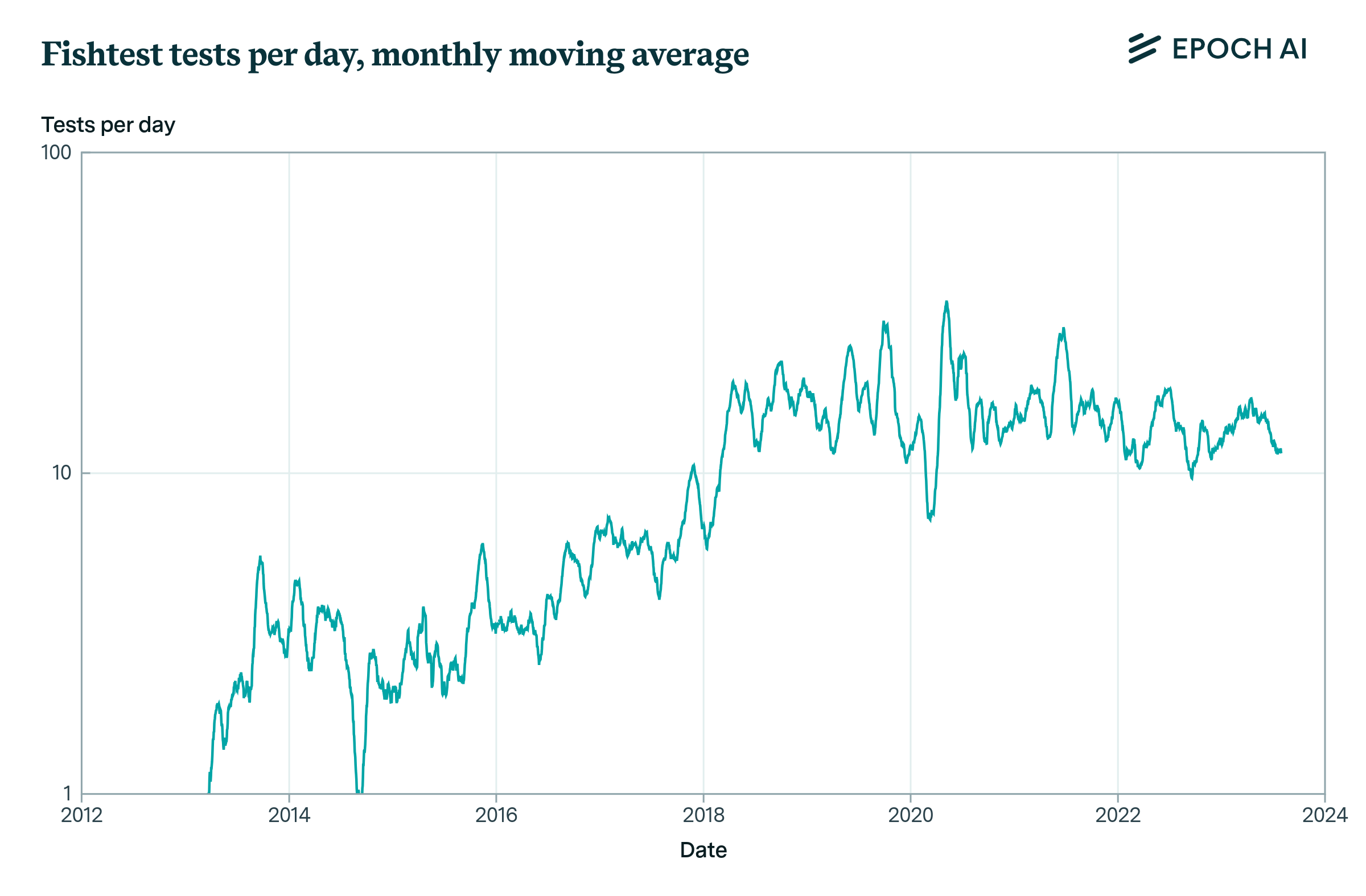
Figure 1: Progress in the algorithmic efficiency of Stockfish over time and number of tests completed on Fishtest per day, averaged over the previous 30 days.
Using the Stockfish data, we obtain a central estimate of returns to research effort, \(r\), of about 0.83, with a standard error of 0.15. This value of \(r\) is just shy of the threshold of \(1\) that we discussed earlier, though our estimates don’t rule out the returns to research effort exceeding unity. If AI R&D is anything like the R&D involved in building better chess engines, then this provides some weak evidence against “foom".
Other domains of software
Unfortunately, in most other domains of software progress, we don’t have the luxury of high-frequency time series data to work with. For example, the best data on R&D outputs only depicts an average rate of software progress over a period of years, and is not informative about fluctuations in software efficiency that may occur across time (Erdil and Besiroglu 2022; Hernandez and Brown 2020).

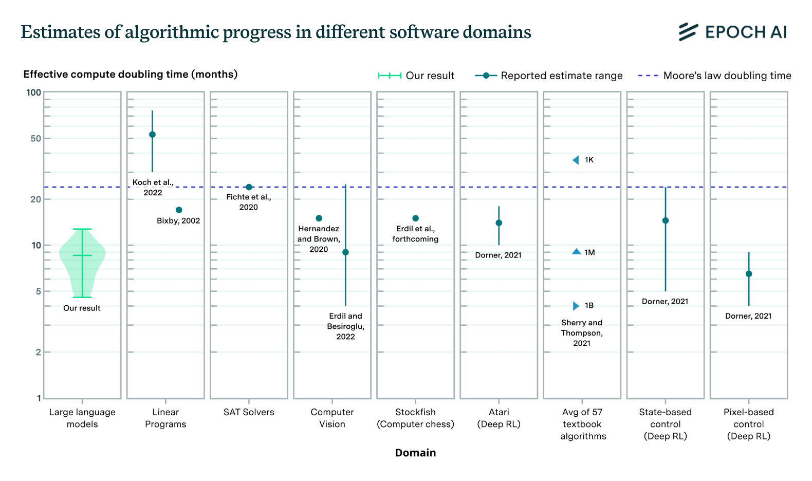
Figure 2: Violin plot of the posterior distributions we obtain for the parameter \(r\) across categories. The \(r=1\) threshold is marked by the dashed horizontal line for ease of viewing, though it does not always have qualitative significance.
To circumvent this issue, we estimate \(r\) using Bayesian inference techniques, where we start with a fairly uninformative prior over parameter values and update based on the limited data available to us. We do this for four domains with estimates of software efficiency \(A\): computer vision, SAT solvers (Fichte, Hecher, and Szeider 2020), linear programming (Koch et al. 2022), and reinforcement learning (Dorner 2021). In each of these cases, the only data available for the output measure is an estimated growth rate in software efficiency. On the input-side, we use estimates of the number of unique authors publishing relevant work.
With this data, our estimation strategy amounts to performing a Bayesian update with a single data point. Clearly this is far from perfect (e.g. because goodness of fit tests cannot be performed if only one data point is available), but it is still preferable compared to previous approaches used in the literature. Our results are shown in Figure 2. In all four of these case studies, our median estimates of \(r\) exceed one, but like in computer chess this finding is not statistically significant. Although these case studies suggest a higher chance of \(r>1\) than for computer chess, we place more weight on our estimates from Stockfish since it’s the domain for which we have the best data. Even still, across these (limited) case studies it appears very plausible that the returns to R&D in software are indeed greater than one.
Note that though the \(r=1\) threshold has been marked by a dashed line in Figure 2, this threshold doesn’t always have a big qualitative significance. This is because not all of the measures of software efficiency in Figure 2 are measures of runtime or inference efficiency. The computer vision data is about training efficiency, while the reinforcement learning data is about sample efficiency. Neither of these are an exact match for the type of progress we need for the model from the section on hyperbolic growth to apply exactly.
Do our estimates point to a singularity?
Our work suggests that the returns to research in software are high – in some cases, our estimates are consistent with a proportional increase in research input resulting in a greater-than-proportional software improvement. In contrast, the returns to R&D in other domains might be substantially lower. For example, Bloom et at. (2020) find a value as low as \(r \approx 0.32\) for the aggregate US economy, and our replication of this result yields an even more pessimistic median estimate of \(r \approx 0.25\). This lends more credence to our previous argument, that if we can automate R&D, and simultaneously scale up the amount of compute used to run AI systems, accelerating growth looks likely.
While our estimates are consistent with the possibility of a software singularity, there are reasons to be cautious in interpreting these results as strong evidence for this outcome. Historically, hardware and software progress have improved at similarly rapid rates, suggesting a symbiotic relationship between the two. One explanation is that hardware advancements enable the exploration of more complex algorithmic ideas, some of which lead to improvements in software efficiency. This implies that software R&D progress might be more challenging without concurrent hardware advancements. Therefore, while our findings are consistent with a software singularity, dependence of software progress on hardware progress could block this possibility.
Conclusion
Our empirical findings presented in our new paper suggest that the returns to software R&D might be high enough to drive hyperbolic growth in software alone, although the evidence is not conclusive. In the case of computer chess—the domain for which we have the most reliable data—our estimates indicate that the key parameter is close to, but slightly below, the threshold required for hyperbolic growth. Estimates for other domains, such as computer vision and reinforcement learning, are less certain due to limited data availability, but they hint at the possibility that a doubling of research inputs may lead to a software singularity.
Historically, improvements in software have been significantly influenced by concurrent advancements in hardware, highlighting a symbiotic relationship between the two. This suggests that software R&D improvements might be more challenging in the absence of parallel hardware progress. Consequently, we do not believe the current empirical data provides strong evidence for the possibility of a software singularity.
It is worth noting that the conditions for a software singularity are considerably stronger than those needed for hyperbolic growth arising from the combined progress in software and hardware. While our findings do not rule out the potential for rapid, potentially hyperbolic improvements in overall capabilities, they do not provide strong evidence that software alone is sufficient to be the sole driver of such growth. Future research should focus on refining empirical methods and obtaining higher quality data to better understand the long-term dynamics of software R&D and its interaction with hardware advancements.
References
Bloom, Nicholas et al. (2020). “Are ideas getting harder to find?” In: American Economic Review 110.4, pp. 1104–1144.
Dorner, Florian E (2021). “Measuring progress in deep reinforcement learning sample efficiency”. In: arXiv preprint arXiv:2102.04881.
Erdil, Ege and Tamay Besiroglu (2022). “Algorithmic progress in computer vision”. In: arXiv preprint arXiv:2212.05153.
Fichte, Johannes K, Markus Hecher, and Stefan Szeider (2020). “A time leap challenge for SAT-solving”. In: Principles and Practice of Constraint Programming: 26th International Conference, CP 2020, Louvain-laNeuve, Belgium, September 7–11, 2020, Proceedings. Springer, pp. 267–285.
Hernandez, Danny and Tom B Brown (2020). “Measuring the algorithmic efficiency of neural networks”. In: arXiv preprint arXiv:2005.04305.
Ho, Anson et al. (2024). Algorithmic progress in language models. arXiv: 2403.05812 [cs.CL].
Jones, Charles I (1995). “R & D-based models of economic growth”. In: Journal of political Economy 103.4, pp. 759–784.
Koch, Thorsten et al. (2022). “Progress in mathematical programming solvers from 2001 to 2020”. In: EURO Journal on Computational Optimization 10, p. 100031.
Stockfish (2023). Useful data. Accessed: July 2023. URL: https://github.com/official-stockfish/Stockfish/wiki/Useful-data##elo-from-speedups
Notes
-
There is a third possible outcome where a proportional increase in AI R&D produces a proportional improvement in AI software, which in turn results in a precisely proportional improvement in subsequent AI-produced R&D output. For the purposes of this exposition, we neglect this knife-edged scenario. ↩
-
The parameter \(\theta\) also influences the long-run dynamics, but only in a quantitative sense (e.g. the value of the exponent under an exponential growth trajectory). In contrast, \(r\) can change the qualitative dynamics of long-run growth, and this will be our primary focus for the purposes of this post. ↩
-
See the literature review in Ho et al. 2024 for some examples of this. ↩
About the authors


Related posts