Trends in the Dollar Training Cost of Machine Learning Systems
I combine training compute and GPU price-performance data to estimate the cost of compute in US dollars for the final training run of 124 machine learning systems published between 2009 and 2022, and find that the cost has grown by approximately 0.5 orders of magnitude per year.
Published
Resources
This report was originally published on Jan 31, 2023. For the latest research and updates on this subject, please see: How Much Does It Cost to Train Frontier AI Models?.
Important caveats about the results in this report
- The cost estimates have large uncertainty bounds—the true costs could be several times larger or smaller. The cost estimates are themselves built on top of estimates (e.g. training compute estimates, GPU price-performance estimates, etc.). See the Methods section and Appendix J for discussion of the uncertainties in the respective estimates.
- Although the estimated growth rates in cost are more robust than any individual cost estimate, these growth rates should also be interpreted with caution—especially when extrapolated into the future.
- The cost estimates only cover the compute for the final training runs of ML systems—nothing more.
- The cost estimates are for notable publicly known ML systems according to the criteria discussed in Sevilla et al. (2022, p.16). The improvements in performance over time are irregular—this means that a 2x increase in compute budget did not always lead to the same improvements in capabilities. This behavior varies widely per domain.
- There’s a big difference in what tech companies pay “internally” and what consumers might pay for the same amount of compute. For example, while Google might pay less per hour for their TPU, they initially carried the cost of developing multiple generations of hardware.
Thanks to Michael Aird, Markus Anderljung, and the Epoch AI team for helpful feedback and comments.
Summary
-
Using a dataset of 124 machine learning (ML) systems published between 2009 and 2022,1 I estimate that the cost of compute in US dollars for the final training run of ML systems has grown by 0.49 orders of magnitude (OOM) per year (90% CI: 0.37 to 0.56).2 See Table 1 for more detailed results, indicated by “All systems.”3
-
By contrast, I estimate that the cost of compute used to train “large-scale” systems since September 2015 (systems that used a relatively large amount of compute) has grown more slowly compared to the full sample, at a rate of 0.2 OOMs/year (90% CI: 0.1 to 0.4 OOMs/year). See Table 1 for more detailed results, indicated by “Large-scale.” (more)
|
Estimation method (go to explanation) |
Data | Period | Scale (start to end)4 | Growth rate in dollar cost for final training runs |
|---|---|---|---|---|
| (1) Using the overall GPU price-performance trend (go to results) |
All systems (n=124) | Jun 2009– Jul 2022 |
$0.02 to $80K | 0.51 OOMs/year 90% CI: 0.45 to 0.57 |
| Large-scale (n=25) | Oct 2015– Jun 2022 |
$30K to $1M | 0.2 OOMs/year5 90% CI: 0.1 to 0.4 |
|
| (2) Using the peak price-performance of the actual NVIDIA GPUs used to train ML systems (go to results) | All systems (n=48) | Jun 2009– Jul 2022 |
$0.10 to $80K | 0.44 OOMs/year6 90% CI: 0.34 to 0.52 |
| Large-scale (n=6)7 | Sep 2016– May 2022 |
$200 to $70K | 0.2 OOMs/year 90% CI: 0.1 to 0.4 |
|
| Weighted mixture of growth rates8 | All systems | Jun 2009– Jul 2022 |
N/A9 | 0.49 OOMs/year 90% CI: 0.37 to 0.56 |
Table 1: Estimated growth rate in the dollar cost of compute to train ML systems over time, based on a log-linear regression. OOM = order of magnitude (10x). See the section Summary of regression results for expanded result tables.
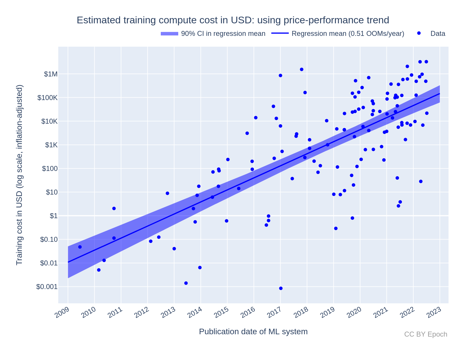
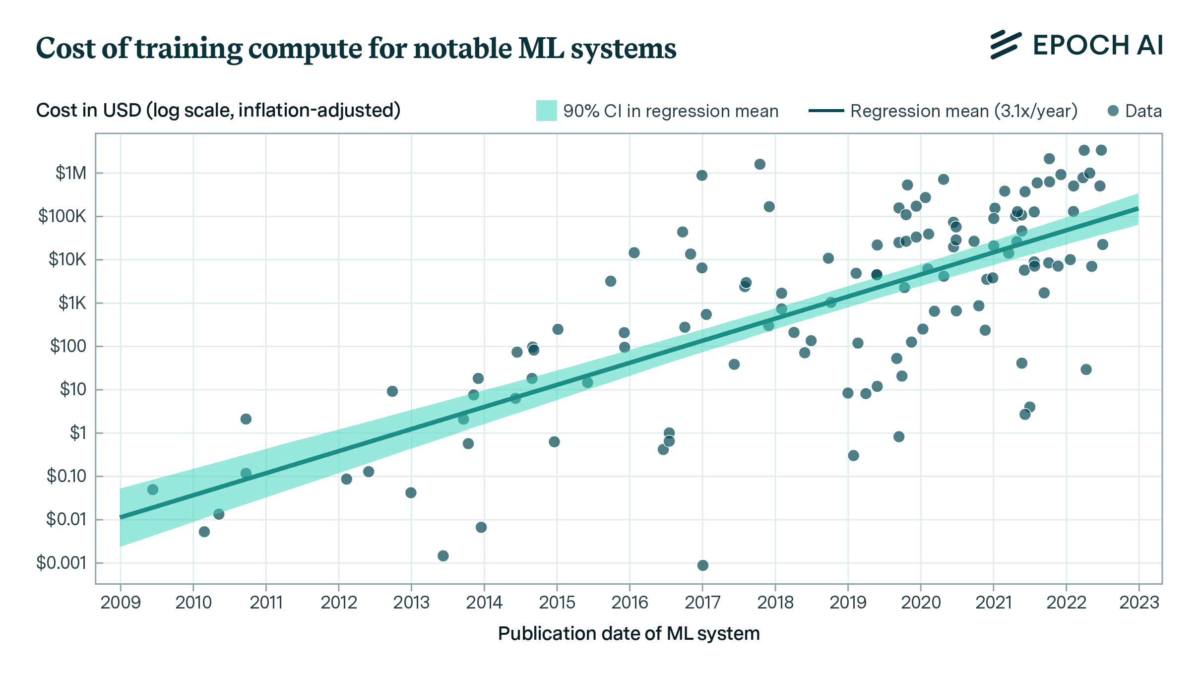
Figure 1: estimated cost of compute in US dollars for the final training run of ML systems. The costs here are estimated based on the trend in price-performance for all GPUs in Hobbhahn & Besiroglu (2022) (known as “Method 1” in this report).
-
I used the historical results to forecast (albeit with large uncertainty) when the cost of compute for the most expensive training run will exceed $233B, i.e. ~1% of US GDP in 2021. Following Cotra (2020), I take this cost to be an important threshold for the extent of global investment in AI.10 (more)
- Naively extrapolating from the current most expensive cost estimate (Minerva at $3.27M) using the "all systems" growth rate of 0.49 OOMs/year (90% CI: 0.37 to 0.56), the cost of compute for the most expensive training run would exceed a real value of $233B in the year 2032 (90% CI: 2031 to 2036).
- By contrast, my best-guess forecast adjusted for evidence that the growth in costs will slow down in the future, and for sources of bias in the cost estimates.11 These adjustments partly relied on my intuition-based judgements, so the result should be interpreted with caution. I extrapolated from the year 2025 with an initial cost of $380M (90% CI: $55M to $1.5B) using a growth rate of 0.2 OOMs/year (90% CI: 0.1 to 0.3 OOMs/year), to find that the cost of compute for the most expensive training run would exceed a real value of $233B in the year 2040 (90% CI: 2033 to 2062).
-
For future work, I recommend the following:
- Incorporate systems trained on Google TPUs, and TPU price-performance data, into Method 2. (more)
- Estimate more reliable bounds on training compute costs, rather than just point estimates. For example, research the profit margin of NVIDIA and adjust retail prices by that margin to get a lower bound on hardware cost. (more)
- As a broader topic, investigate trends in investment, spending allocation, and AI revenue. (more)
Why study dollar training costs?
The cost of compute (in units of FLOP) for ML training runs is useful to understand how ML capabilities develop over time. For instance, estimates of compute cost can be combined with performance metrics to measure the efficiency of ML systems over time. However, due to Moore’s Law (and more specifically, hardware price-performance trends), computational costs have become exponentially cheaper (in dollars) over time. In the past decade, growth in compute spending in ML has been much faster than Moore’s Law.12
In contrast to compute, the dollar cost of ML training runs is more indicative of how expensive (in real economic terms) those training runs are, and an actor’s willingness to spend on those training runs. Understanding dollar costs and the willingness to spend can in turn help with forecasting
- The rate of AI progress (due to the dependence of AI development on economic factors, rather than just the innate difficulty of research progress).
- Which actors can financially afford to develop Transformative AI (TAI), which in turn informs which actors will be first to develop TAI.
The primary aim of this work is to address the following questions about training costs:
- What is the growth rate in dollar training cost over time?
- Is the training cost trend stable, slowing down, or speeding up?
- What are the most expensive ML training runs to date?
An additional aim is to explore different methods to estimate the dollar cost and analyze the effect of differences between the methods. I think it is particularly important to explore alternative estimation methods as a way of reducing uncertainty, because there tends to be even less publicly available information about the dollar cost of ML training runs than the compute cost.
Method
Background on methods to estimate the dollar cost of training compute
In this work, I estimate the actual cost of compute for the final training run that produced a given ML system.13 I break down the cost of compute for the final training run into
- Hardware cost: the portion of the up-front cost of hardware spent on the training run.
- Energy cost: the cost of electricity to power the hardware during the training run.
To estimate hardware cost, the simplest model I am aware of is:14
\[ \textit{hardware_cost} = \frac{\textit{training_time}}{\textit{hardware_replacement_time}} \cdot \textit{n_hardware} \cdot \textit{hardware_unit_price} \]
where training_time is the number of GPU hours used per hardware unit for training, and hardware_replacement_time is the total number of GPU hours that the hardware unit is used before being replaced with new hardware.
The model here is that a developer buys n_hardware units at hardware_unit_price and uses each hardware unit for a total duration of hardware_replacement_time. So the up-front cost of the hardware is amortized over hardware_replacement_time, giving a value in $/s for using the hardware. The developer then spends training_time training a given ML system at that $/s rate. Note that this neglects hardware-related costs other than the sale price of the hardware, e.g., switches and interconnect cables.
To estimate energy cost, the simplest model I am aware of is:15
\[ \textit{energy_cost} = \textit{training_time} \cdot \textit{n_hardware} \cdot \textit{hardware_power_consumption} \cdot \textit{energy_rate} \]
Where hardware_power_consumption is in kW and energy_rate is in $/kWh. Maximum power consumption is normally listed in hardware datasheets—e.g., the NVIDIA V100 PCIe model is reported to have a maximum power consumption of 0.25kW.
Using cloud compute prices provides a way to account for hardware, energy and maintenance costs without estimating them individually. Cloud compute prices are normally expressed in $ per hour of usage and per hardware unit (e.g., 1 GPU).16 So to calculate the cost of computing the final training run with cloud computing, one can just use
\[ \textit{training_cost} = \textit{training_time} \cdot \textit{n_hardware} \cdot \textit{cloud_computing_price} \]
However, because cloud compute vendors need to make a profit, the cloud computing price would also include a margin added to the costs of the vendor. For this reason, cloud computing prices (especially on-demand rather than discounted prices) are useful as an upper bound on the actual training cost. In this work, I only estimate costs using hardware prices rather than cloud compute prices.
Estimating training cost from training compute and GPU price-performance
The estimation models presented in the previous section seem to me like the simplest models, which track the variables that are most directly correlated with cost (e.g., the number of hardware units purchased). Those models therefore minimize sources of uncertainty. However, information about training time and the number of hardware units used to train an ML system is often unavailable. On the other hand, information that is sufficient to estimate the training compute of an ML system is more often available. Compute Trends Across Three Eras of Machine Learning (Sevilla et al., 2022) and its accompanying database17 provide the most comprehensive set of estimates of training compute for ML systems to date.18 Due to the higher data availability, I chose an estimation model that uses the training compute in FLOP, rather than the models presented in the previous section.
To estimate the hardware cost from training compute, one also needs to know the price-performance of the hardware in FLOP/s per $. In this work, I use the price-performance trend found for all GPUs (n=470) in Trends in GPU price-performance. I also use some price-performance estimates for individual GPUs from the dataset of GPUs in that work (see this appendix for more information). I only estimate hardware cost and not energy cost. This is because (a) energy cost seems less significant (see this appendix for evidence), and (b) data related to hardware throughput and compute was more readily available to me than data on energy consumption.
The actual model I used to estimate the hardware cost of training (in $) for a given ML system was:
\[ \textit{hardware_cost} = \textit{training_compute} / \textit{realised_training_compute_per_\$} \]
where realised_training_compute_per_$ is in units of FLOP/$:
\[ \textit{realised_training_compute_per_\$} = \textit{hardware_price_performance} \cdot \textit{hardware_utilization_rate} \cdot \textit{hardware_replacement_time} \]
Where hardware_utilization_rate is the fraction of the theoretical peak FLOP/s throughput that is realized in training. The hardware_price_performance is in FLOP/s per $:
\[ \textit{hardware_price_performance} = \textit{peak_throughput} / \textit{hardware_unit_price} \]
There are several challenges for this model in practice:
-
Training compute is itself an estimate based on multiple variables, and tends to have significant uncertainty.19
- Hardware replacement time varies depending on the resources and needs of the developer. For example, a developer may upgrade their hardware sooner due to receiving enough funding to perform a big experiment, even though they haven’t “paid off” the cost of their previous hardware with research results.
- Information on the hardware utilization rate achieved for a given ML system is often unreliable.
- Hardware unit prices vary over time—in recent years (since 2019), fluctuations of about 1.5x seem typical.20
I made the following simplifying assumptions that neglect the above issues:
- The training compute estimate is the true value.
- Hardware replacement time is constant at two years.21
- A constant utilization rate of 35% was achieved during training.22
- For each hardware model, I used whatever unit price I could find that was reported closest to the release date of the hardware, as long as it was reported by a seemingly credible source. (More information on data sources is in this appendix.)
Although the results in this work rely on the above assumptions, I attempted to quantify the impact of the assumptions in this appendix to estimate my actual best guess and true uncertainty about the cost of compute for the final training runs of ML systems.
Method 1: Using the overall GPU price-performance trend
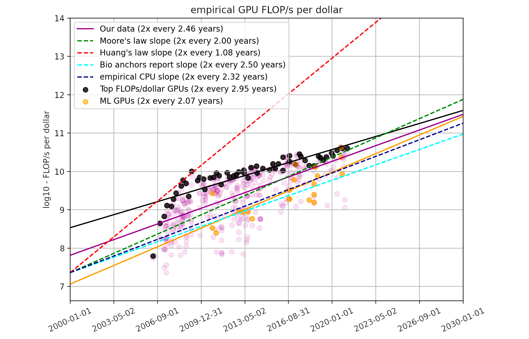
One way of estimating the hardware_price_performance variable is to use the overall trend in price-performance over time. This saves from needing to know the actual hardware used for each ML system. Trends in GPU price-performance estimated that on average, the price-performance of GPU hardware in FLOP/s per $ has doubled approximately every 2.5 years. I used this trend as my first method of estimating price-performance. In particular, I calculated price-performance as the value of the trend line at the exact time an ML system was published.
Method 2: Using the price-performance of actual hardware used to train ML systems
Method 1 is unrealistic in the following ways:
- The purchase of hardware would actually happen before the publication date of the system, perhaps months or years before the training run started.
- The actual price-performance that can be achieved is discrete.
- Firstly, price-performance depends on which GPUs are available at a given time. The time at which new GPUs become available is discrete and somewhat irregular, as seen in the plots in Trends in GPU price-performance.
- Secondly, price-performance depends on the actual choice of hardware. The actual price-performance varies depending on the specific hardware model, and the hardware that was actually used may be older than the latest available hardware on the market.
In an effort to address these limitations, my second estimation method is based on the price-performance of the actual hardware used to train a given ML system. For example, GPT-3 was reported to use NVIDIA V100 GPUs. So to estimate the training cost of GPT-3, I used the actual FLOP/s specification of the V100, and its estimated unit price, to calculate the price-performance in FLOP/s per $. I then used that price-performance value in the hardware cost formula above.
Dataset
My dataset is available at Training cost trends in machine learning. Details of how the data were collected and processed are in this appendix.
Code
All results were produced using the accompanying Colab notebook.
Large-scale systems
The main results presented in Compute Trends Across Three Eras of Machine Learning involved splitting one compute trend into two simultaneous trends from late 2015 onwards. One of these trends was for “large-scale” systems—systems that were outliers above the mean compute trend for all systems (i.e., systems that used an abnormally high amount of training compute). Given the relationship between training compute and AI capabilities,23 the trend for these large-scale systems can better inform what the frontier of AI capabilities will be at future times.
To get a dataset of training costs for large-scale systems, I started with the same set of systems as Compute Trends Across Three Eras of Machine Learning. I then added the following systems that were released more recently, based on visual inspection of the plot presented in this results section:24 ‘Chinchilla,’ ‘PaLM (540B),’ ‘OPT-175B,’ ‘Parti,’ and ‘Minerva (540B).’
Results
Method 1: Using the overall GPU price-performance trend for all ML systems (n=124)
Growth rate of training cost for all ML systems: 0.51 OOMs/year
Figure 2 plots the training cost of the selected ML systems (n=124) against the system’s publication date, with a linear trendline (note the log-scaled y axis). Applying a log-linear regression, I find a growth rate of 0.51 OOMs/year (90% CI: 0.45 to 0.57 OOMs/year) in the dollar cost of compute for final training runs. Notably, this trend represents slower growth than the 0.7 OOMs/year (90% CI: 0.6 to 0.7 OOMs/year) for the 2010 – 2022 compute trend in FLOP for “all systems” (n=98) in Sevilla et al. (2022, Table 3).
Note that this estimate of growth rate is just a consequence of combining the log-linear trends in compute and price-performance. A similar growth rate can be estimated simply by taking the growth rate in compute (0.7 OOMs/year) and subtracting the growth rate in GPU price-performance (0.12 OOMs/year), as reported in prior work.25
Based on the fitted trend, the predicted growth in training cost for an average milestone ML system by the beginning of 2030 is:
- +3.6 OOMs (90% CI: +3.2 to +4.0 OOMs) relative to the end of 2022
- $500M (90% CI: $90M to $3B)
Here, and in all subsequent results like the above, I am more confident in the prediction of additional growth in OOMs than the prediction of exact cost, because the former is not sensitive to any constant factors that may be inaccurate, e.g., the hardware replacement time and the hardware utilization rate.
Figure 2: Estimated training compute cost of milestone ML systems using the continuous GPU price-performance trend. See this Colab notebook cell for an interactive version of the plot with ML system labels.
Growth rate of training cost for large-scale ML systems: 0.2 OOMs/year
After fitting a log-linear regression to the “large-scale” set of systems, I obtained the plot in Figure 3. The resulting slope was approximately 0.2 OOMs/year (90% CI: 0.1 to 0.4 OOMs/year). While this result is based on a smaller sample (n=25 compared to n=124), I think the evidence is strong enough to conclude that the cost of the most expensive training run is growing significantly slower than milestone ML systems as a whole. This is consistent with the direction of predictions in AI and Compute (from CSET), and Cotra’s “Forecasting TAI with biological anchors”26—namely, that recent growth spending will likely slow down greatly during the 2020s, given the current willingness of leading AI developers to spend on training, and given that the recent overall growth rate seems unsustainable.
Clearly, the growth rate of large-scale systems cannot be this much lower than the growth rate of all systems for long—otherwise, the growth in all systems would quickly overtake the current large-scale systems. The main reason that the large-scale growth is much slower seems to be that the selection of “large-scale” systems puts more weight on high-compute outliers. Outliers that occurred earlier in this dataset such as AlphaGo Master and AlphaGo Zero are particularly high, which makes later outliers look less extreme. However, I don’t think this undercuts the conclusion that spending on large-scale systems has grown at a slower rate; rather, it adds uncertainty about the future costs of large-scale systems.
Based on the fitted trend, the predicted growth in training cost for a large-scale ML system by the beginning of 2030 is:
-
+1.8 OOM (90% CI: +1.0 to +2.4 OOM) relative to the end of 2022.27
-
$80M (90% CI: $6M to $700M)
So although the large-scale trend starts higher than the average trend for all systems (see the previous section), the slower growth leads to a lower prediction than $500M (90% CI: $100M to $3B).
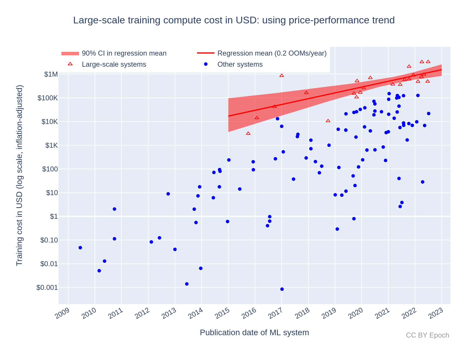
Figure 3: Estimated training compute cost of large-scale ML systems using Method 1. See this Colab notebook cell for an interactive version of the plot with ML system labels.
Method 2: Using the price-performance of NVIDIA GPUs used to train ML systems (n=48)
Growth rate of training cost for all ML systems: 0.44 OOMs/year
Figure 4 plots the order-of-magnitude of training cost of ML systems trained with NVIDIA GPUs (n=48) against the system’s publication date, with a linear trendline. I find a trend of 0.44 OOMs/year (90% CI: 0.34 to 0.52). So this model predicts slower growth than the model based on the overall GPU price-performance trend, which was 0.51 OOMs/year (90% CI: 0.44 to 0.59). It turns out that this difference in growth rate (in OOMs/year) is merely due to the smaller dataset, even though the estimates of absolute cost (in $) are roughly twice as large as those of Method 1 on average.28
Based on the fitted trend, the predicted growth in training cost for an average milestone ML system by the beginning of 2030 is
- +3.1 OOM (90% CI: +2.4 to +3.6 OOM) relative to the end of 2022
- $200M (90% CI: $8M to $2B)
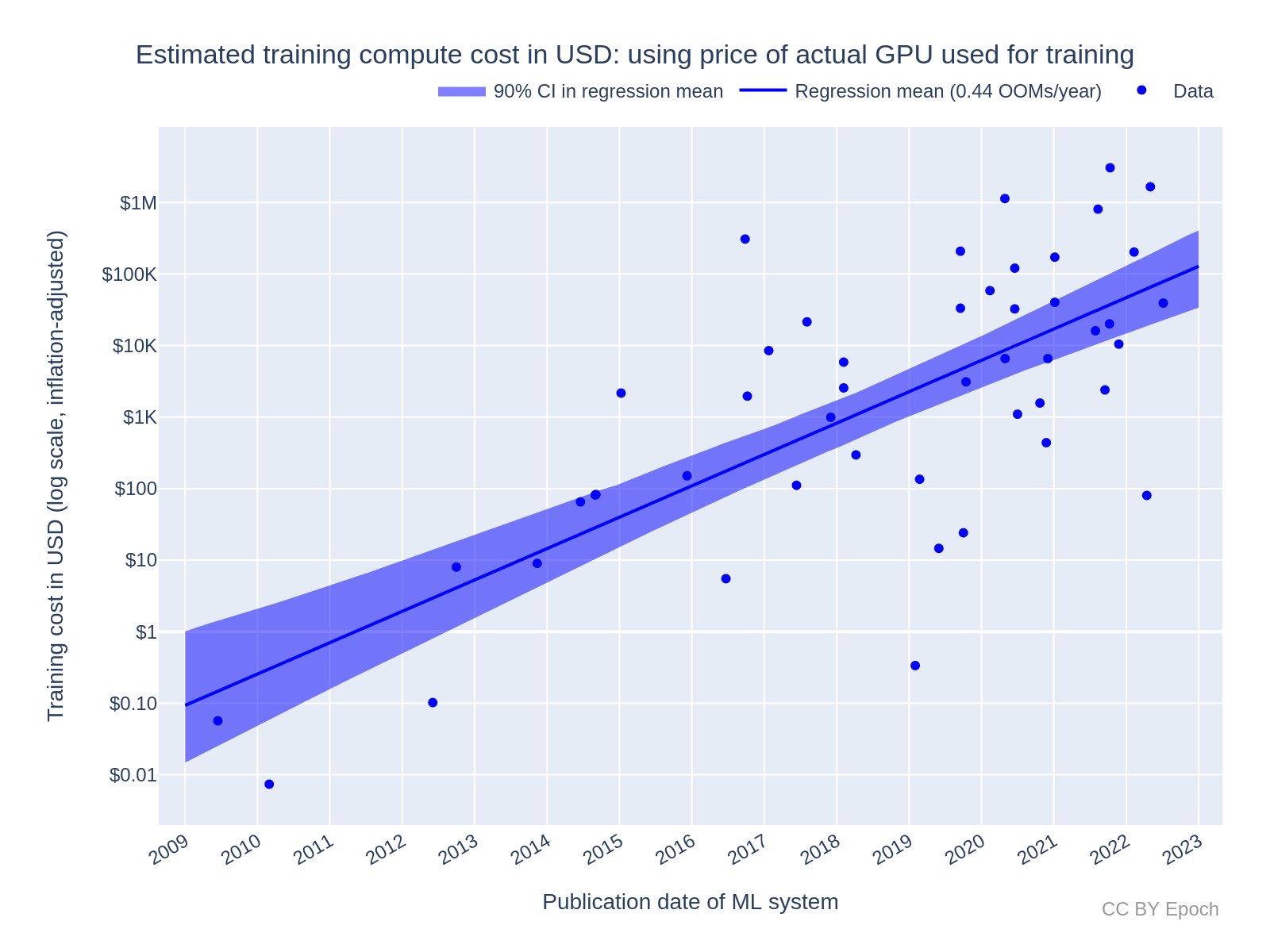
Figure 4: Estimated training compute cost of milestone ML systems using the peak price-performance of the actual NVIDIA GPUs used in training. See this Colab notebook cell for an interactive version of the plot with ML system labels.
Growth rate of training cost for large-scale ML systems: 0.2 OOMs/year
For the trend in large-scale systems, I used the same method to filter large-scale systems as in Method 1, but only included the systems that were in the smaller Method 2 sample of n=48. This left only 6 systems. After fitting a log-linear regression to this set of systems, I obtained the plot in Figure 5. The resulting slope was approximately 0.2 OOMs/year (90% CI: 0.1 to 0.4 OOMs/year). The sample size is very small and the uncertainty is very large, so this result should be taken with a much lower weight than other results. I think the prediction that this regression makes for 2030 should be disregarded in favor of Method 1. However, the result is at least consistent with Method 1 in suggesting that the cost of the most expensive training run has been growing significantly slower than milestone ML systems as a whole.
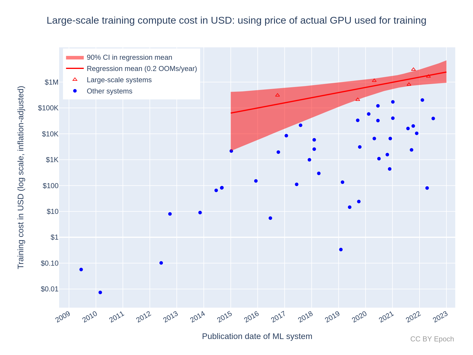
Figure 5: Estimated training compute cost of large-scale ML systems using Method 2. See this Colab notebook cell for an interactive version of the plot with ML system labels.
Summary and comparison of all regression results
Table 2 and Table 3 summarize all of the regression results for “All systems” and “Large-scale” systems, respectively. Based on an analysis of how robust the regression results for “All systems” are to different date ranges, the mean growth rate predicted by Method 1 seems reasonably robust across different date ranges, whereas Method 2 is much less robust in this way (see this appendix for more information). However, I believe that the individual cost estimates via Method 2 are more accurate, because Method 2 uses price data for the specific hardware used to train each ML system. Overall, I think the growth rate obtained via Method 1 is more robust for my current dataset, but that conclusion seems reasonably likely to change if a comparable number of data points are acquired for Method 2. Collecting that data seems like a worthwhile task for future work.
| Estimation method | Period | Data | Growth rate (OOMs/year) | Predicted average cost by 2030 |
|---|---|---|---|---|
| Method 1 (using average trend in hardware prices) | 2009– 2022 |
All systems (n=124) | 0.51 90% CI: 0.45 to 0.57 |
$500M (90% CI: $90M to $3B) |
| Method 2 (using actual hardware prices) | 2009– 2022 |
All systems (n=48) | 0.44 OOMs/year 90% CI: 0.34 to 0.52 |
$200M (90% CI: $8M to $2B) |
| Weighted mixture of results29 | 2009– 2022 |
All systems | 0.49 OOMs/year 90% CI: 0.37 to 0.56 |
$350M (90% CI: $40M to $4B)30 |
| Compute trend (for reference)31 | 2010– 2022 |
All systems (n=98) | 0.7 OOMs/year 95% CI: 0.6 to 0.7 |
N/A |
| GPU price-performance trend (for reference)32 | 2006– 2021 |
All GPUs (n=470) | 0.12 OOMs/year 95% CI: 0.11 to 0.13 |
N/A |
Table 2: Estimated growth rate in the dollar cost of compute for the final training run of milestone ML systems over time, based on a log-linear regression. For reference, the bottom two rows show trends in training compute (in FLOP) and GPU price-performance (FLOP/s per $) found in prior work.
| Estimation method | Period | Data | Growth rate (OOMs/year) | Predicted average cost by 2030 |
|---|---|---|---|---|
| Method 1 (using average trend in hardware prices) | 2015–2022 | Large-scale (n=25) | 0.2 OOMs/year 90% CI: 0.1 to 0.4 |
$80M (90% CI: $6M to $700M) |
| Method 2 (using actual hardware prices) | 2015–2022 | Large-scale (n=6) | 0.2 OOMs/year 90% CI: 0.1 to 0.4 |
$60M (90% CI: $2M to $9B) |
| Compute trend (for reference)33 | 2015–2022 | Large-scale (n=16) | 0.4 OOMs/year 95% CI: 0.2 to 0.5 |
N/A |
Table 3: Estimated growth rate in the dollar cost of compute for the final training run of large-scale ML systems over time, based on a log-linear regression. The bottom row shows the trend in training compute (in FLOP) found in prior work, for reference.
Predictions of when a spending limit will be reached
The historical trends can be used to forecast (albeit with large uncertainty) when the spending on compute for the most expensive training run will reach some limit based on economic constraints. I am highly uncertain about the true limits to spending. However, following Cotra (2020), I chose a cost limit of $233B (i.e. 1% of US GDP in 2021) because this at least seems like an important threshold for the extent of global investment in AI.34
I used the following facts and estimates to predict when the assumed limit would be reached:
- US GDP: $23.32 trillion in 202135
- Chosen threshold of spending: 1% of GDP = 0.01 * $23.32T = $233.2B
- This number is approximately equal to 10^11.37
- Historical starting cost estimate: $3.27M (Minerva)
- This number is approximately equal to 10^6.51
- Minerva occurs at approximately 2022.5 years (2022-Jun-29)
- Estimated cost at the beginning of 2025: $60M36
- This is approximately 10^7.78
- Formula to estimate the year by which the cost would reach the spending limit: [starting year] + ([ceiling] - [start] in OOMs) / [future growth rate in OOMs/year]
- An example using numbers from above: 2022.5 + (11.37 - 6.51 OOMs) / (0.49 OOMs/year) ~= 2032
These were my resulting predictions, first by naive extrapolation and then based on my best guess:
- Naively extrapolating from the current most expensive cost estimate (Minerva, $3.27M) using historical growth rates:
- Using the “all systems” trend of 0.49 OOMs/year (90% CI: 0.37 to 0.56), a cost of $233.2B would be reached in the year 2032 (90% CI: 2031 to 2036). This extrapolation is illustrated in Figure 6.
- Using the “large scale” trend of 0.2 OOMs/year (90% CI: 0.1 to 0.4), a cost of $233.2B would be reached in the year 2047 (90% CI: 2035 to 2071).
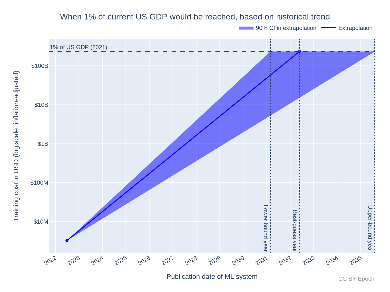
Figure 6: Extrapolation of training cost to 1% of current US GDP, based only on the current most expensive cost estimate (Minerva, $3.27M) and the historical growth rate found for “all systems”.
-
My best guess adjusts for evidence that the growth in costs will slow down in the future, and for sources of bias in the cost estimates.37 These adjustments partly rely on my intuition-based judgements, so the results should be interpreted with caution. The results are38:
-
Independent impression39: extrapolating from the year 2025 with an initial cost of $200M (90% CI: $29M to $800M) using a growth rate of 0.3 OOMs/year (90% CI: 0.1 to 0.4 OOMs/year), a cost of $233.2B would be reached in the year 2036 (90% CI: 2032 to 2065).
-
All-things-considered view: extrapolating from the year 2025 with an initial cost of $380M (90% CI: $55M to $1.5B) using a growth rate of 0.2 OOMs/year (90% CI: 0.1 to 0.3 OOMs/year), a cost of $233.2B would be reached in the year 2040 (90% CI: 2033 to 2062). This extrapolation is illustrated in Figure 7.
-
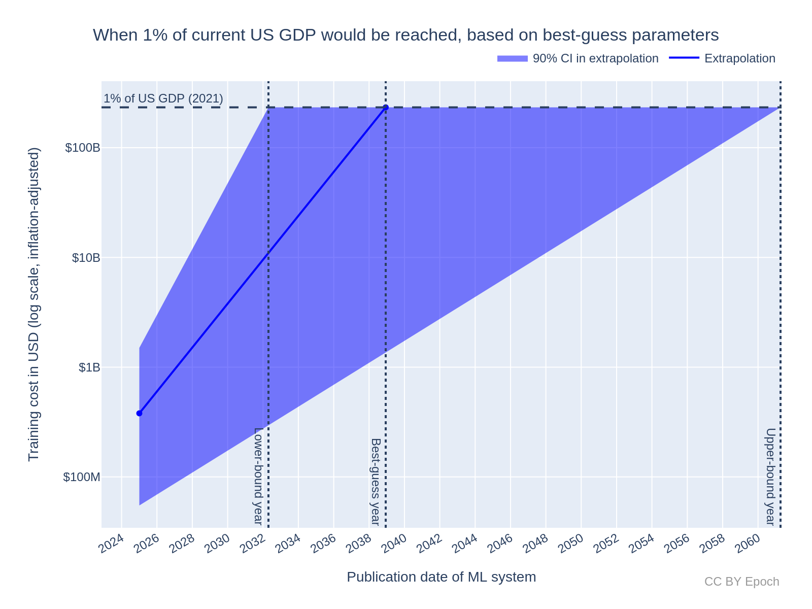
Figure 7: Extrapolation of training cost to 1% of current US GDP, based on my best-guess parameters for the most expensive cost in 2025 and the growth rate. Note that the years I reported in the text are about 1 year later than the deterministic calculations I used in this plot—I suspect this is due to the Monte Carlo estimation method used in Guesstimate.
Recommended future work
Include systems trained with Google TPUs for Method 2
The dataset used for Method 2 only had 48 samples, compared to 124 samples for Method 1. Furthermore, the dataset only included ML systems that I could determine to be trained using NVIDIA GPUs. Future work could include other hardware, especially Google TPUs, which I found were used to train at least 25 of the systems in my dataset (some systems have missing data, so it could be more than 25).
Estimate more reliable bounds on cost using cloud compute prices and profit margins
For future work I recommend estimating more reliable bounds on FLOP/$ (and in turn the hardware cost of training runs) by extending the following methods:40
- FLOP/$ estimation method 1: Dividing the peak performance of the GPU (in FLOP/s) by its price (in $) to get the price-performance. Multiplying that by a constant hardware replacement time (in seconds) to get a value in FLOP/$.
- Extension 1: estimate the profit margin of NVIDIA for this GPU. Adjust the reported/retail price by that margin to get a lower bound on hardware cost (i.e., basically the manufacturing cost). Then use that cost instead of the reported/retail price to get an upper-bound value of FLOP/s per $ which can be used in Method 1.
- This can provide a lower bound on training compute cost, because the hardware is as cheap as possible.
- Extension 2: divide the reported/retail price (or the estimated manufacturing cost, as in Extension 1) in $ by the cloud computing rental prices in $/hour to estimate the hardware replacement time. Then use that value in Method 1.
- If the manufacturing cost is a lower bound on price, and on-demand cloud computing rental prices are an upper bound on price per hour, then this gives a lower bound on hardware replacement time.
- Using the retail price and the maximally discounted rental price (e.g., the discount for a three-year rental commitment) would instead make this estimate closer to an upper bound on hardware replacement time.
- Extension 1: estimate the profit margin of NVIDIA for this GPU. Adjust the reported/retail price by that margin to get a lower bound on hardware cost (i.e., basically the manufacturing cost). Then use that cost instead of the reported/retail price to get an upper-bound value of FLOP/s per $ which can be used in Method 1.
- FLOP/$ estimation method 2: Dividing the peak performance of the GPU (FLOP/s) by its current cloud computing rental cost ($/hour) to get a value in FLOP/$.
- Extension 1: extrapolate from this present FLOP/$ value into the past at time t (the publication date of the ML system), using the overall GPU price-performance growth rate. Here we assume that FLOP/$ and FLOP/s per $ differ only by a constant factor, so the growth rate is the same for FLOP/$ and FLOP/s per $.
- Using the resulting FLOP/$ value then gives an upper bound on training compute cost, because on-demand hourly cloud compute prices have a relatively large profit margin, and I expect that any ML systems in my dataset which were trained with cloud compute were very likely to take advantage of the discounts that are offered by cloud computing services.41
- Extension 1: extrapolate from this present FLOP/$ value into the past at time t (the publication date of the ML system), using the overall GPU price-performance growth rate. Here we assume that FLOP/$ and FLOP/s per $ differ only by a constant factor, so the growth rate is the same for FLOP/$ and FLOP/s per $.
Investigate investment, allocation of spending, and revenue
An important broad topic for further investigation is to understand the trends of and the relationships between investment in AI, the allocation of spending on AI, and revenue generated by AI systems. This would inform estimates of the willingness to spend on AI in the future, and whether the growth rate in large-scale training compute cost will continue to decrease, remain steady, or increase. This in turn informs forecasts of when TAI will arrive, and what the impacts of AI will be in the meantime.
Appendices
Appendix A: The energy cost of final training runs seems about 20% as large as the hardware cost
As an example of energy cost, GPT-3 is estimated to have consumed 1,287 MWh of energy during training.42 This estimate is based on the measured system average power per GPU chip, including memory, the network interface, cooling fans, and the host CPU. This estimate also accounts for the “energy overhead above and beyond what directly powers the computing equipment inside the datacenters.”43 The average US energy price in 2020 was approximately $0.13 per kWh, judging by the first plot in this article from the US Energy Information Administration. Multiplying these numbers gives 1,287,000 kWh * $0.13/kWh = $167,310.
For comparison, my estimate of GPT-3’s hardware cost was
- $700K using the overall linear trend of GPU price-performance
- $1.1M using the price-performance of the actual hardware
So the energy cost is about 24% or 15% of the hardware cost (which averages to approximately 20%, the headline figure in the title). Energy cost would make up about 20% or 13% of the combined energy and hardware cost of training, respectively (which averages to approximately 17%).
Note that this is only one example, using one machine learning model, but I think it provides an informative ballpark figure for energy cost relative to hardware cost. Based on this one example, I assume that hardware cost is generally several times larger than energy cost, and is therefore more important to focus on when estimating the total cost to produce machine learning systems.
Appendix B: Data collection and processing
I sourced the names of ML systems, their publication date, and their training compute costs in FLOP from Parameter, Compute and Data Trends in Machine Learning (as of August 20, 2022).44 The systems in that database were considered “milestone” ML systems.45 I filtered the list of systems down to those which had existing estimates of compute cost in FLOP, and were published after 2006 (since this is roughly when the GPU price-performance data begins). This left me with 124 systems. The earliest system is “GPU DBNs” from “Large-scale Deep Unsupervised Learning using Graphics Processors” released in 2009, which happens to be just before the Deep Learning era began in 2010.46
For Method 1, I used the trend for all GPUs reported in Trends in GPU price-performance (i.e., a doubling time of 2.45 years, or a 10x time of 8.17 years). Since their data goes up to 2020 and adjusts for inflation,47 I used units of 2020 USD for dollar training cost. I also included ML systems from 2021 and 2022, whereas the GPU price-performance data only goes to 2021, so I am extrapolating that trend slightly.
Data on the hardware used to train each ML system is in the “Hardware model” column of my dataset’s “ML SYSTEMS” column. Out of the 124 ML systems, I found 78 systems that had specific hardware information in the publication.48 Of these 78 systems, 48 used NVIDIA GPUs. For the “actual hardware” estimation method (AKA Method 2), the sample included just the 48 systems that used NVIDIA GPUs. Future work could include other hardware such as Google TPUs, which I found were used to train at least 25 of the systems in my dataset.49
To estimate the price-performance of individual hardware models, I constructed a spreadsheet called “HARDWARE” which can be found in the dataset linked above. Initially, this was a copy of the “HARDWARE_DATA” sheet in the Parameter, Compute and Data Trends in Machine Learning database, but I made several modifications:
- Added more GPUs or more data about GPUs, including the NVIDIA A100
-
Added more sources of price information and combined those sources to get one estimate of price50
- Added a “Peak FP performance (FLOP/s)” column
The “Peak FP performance (FLOP/s)” column represents the maximum theoretical performance that is offered by the hardware. For NVIDIA accelerator GPUs, peak performance with floating point numbers is achieved when operating in “Tensor” or “Tensor Core” mode. This mode uses mixed precision in its number representations, e.g., FP16 with FP32 accumulation. Where specific peak performance is unavailable, this column defaults to the maximum of the floating-point performance values in other columns. I then estimated price-performance for actual hardware models by dividing the peak performance by an estimated unit price to get a FLOP/s per $ value.51
I used the maximum (peak) performance specified for each GPU rather than a consistent type of performance (e.g., 32-bit number representation) so that the cost estimates are more reflective of the best performance that ML developers could have achieved. However, note that I still adjusted this peak performance down by multiplying the peak value by a hardware utilization rate of 35%. Using peak performance leads to a lower cost estimate than otherwise.
Appendix C: Regression method
All reported regression results were obtained from a bootstrap with 1000 samples. The mean estimate of the growth rate in cost (in OOMs/year) was the mean slope of the regression, averaged over the bootstrap samples. The 90% CI in the growth rate was the 5th and 95th percentile of the slope of the regression obtained in the bootstrap samples. I calculated the projections of the regression (e.g., the “Predicted average cost by 2030” column in Table 2) by calculating the projection within each bootstrap sample, and then taking the mean/5th percentile/95th percentile of the samples. For the exact implementations, see this Colab notebook cell.
I also accounted for uncertainty in the estimated training compute (in FLOP) using the same process as Sevilla et al. (2022, Appendix A). In each bootstrap sample, I multiplied the compute for each ML system by a factor that was randomly and independently sampled from a log-uniform distribution between 0.5 and 2. However, the presence of these random multipliers did not have a significant impact on the estimates of growth rates.52
Differences to Sevilla et al. (2022)
Compute Trends Across Three Eras of Machine Learning (Sevilla et al., 2022) looked at trends in the amount of compute (in FLOP) used to train milestone ML systems over time. Since training compute is one of the key variables in my estimation models of the training cost in dollars, a lot of my analysis is similar to Sevilla et al. (2022). However, I made some independent decisions in my approach, and the following differences are worth noting:
-
I included low-compute outliers in the compute dataset when analyzing trends in the dollar cost, because I wasn’t confident enough in reasons to exclude these systems.53
-
I included AlphaGo systems in my dataset of the most expensive systems (but I did not do a regression on that dataset, which Sevilla et al. did).54 While AlphaGo systems may be statistical outliers, I think that the first transformative AI systems are likely to be (close to) the most expensive systems ever trained, and the AlphaGo systems provide a precedent for that.
- My dataset includes more systems that were added to the Parameter, Compute and Data Trends in Machine Learning database since Sevilla et al. (2022) was published, e.g., Minerva.
- I exclude “Pre Deep Learning Era” data from consideration, except for the system called “GPU DBNs.” This sole exception is due to how I selected data (see the appendix on data sources).
- Method 2 to estimate training cost excludes a majority of systems that were included in Sevilla et al. (2022), due to the availability of data about training hardware.
Appendix D: Inspecting the price-performance of NVIDIA GPUs as a function of ML system publication date
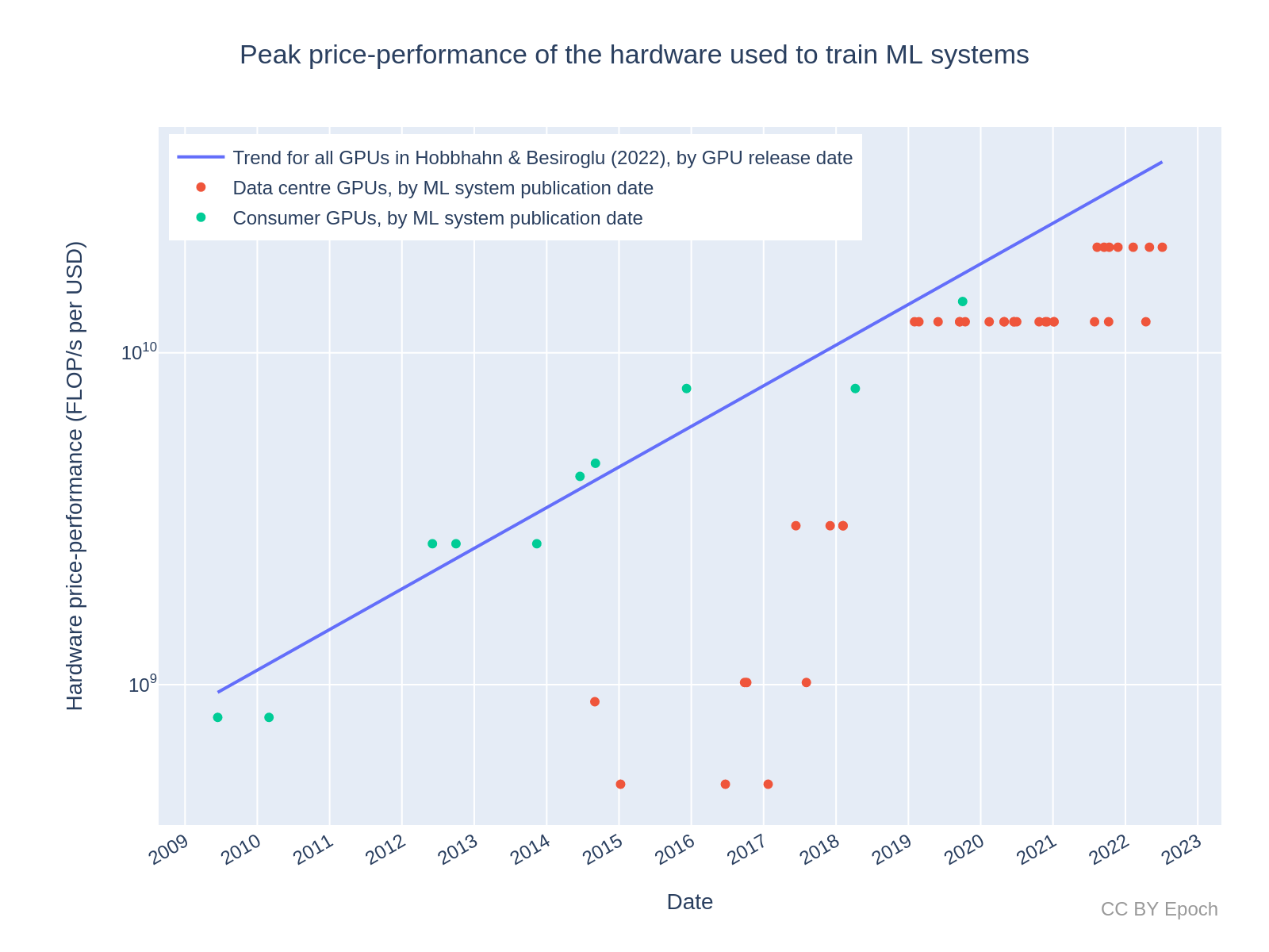
Figure 7: Peak price-performance of NVIDIA GPUs used to train ML systems, separated into data center GPUs (e.g., NVIDIA A100) and consumer GPUs (e.g., NVIDIA GeForce GTX TITAN). See this Colab notebook cell for an interactive version of the plot with ML system and hardware labels.
From a visual inspection of Figure 7, the timing of ML systems that were trained using NVIDIA’s consumer GPUs (i.e., the NVIDIA GeForce GTX series) keeps pace with the trend of GPU price-performance (indicated by the blue line). The delays between the hardware release date and the ML system publication date do not seem to affect this significantly. Meanwhile, the timing of ML systems that were trained using NVIDIA data center GPUs (the K-, P- and V- models) lag behind the trend much more. The price-performance of these GPUs is about 2.5x lower than the trendline on average.55 However, the latest data center GPUs (V100 and A100) start much closer to the trend line than earlier data center GPUs. Overall, this data explains why Method 2 tends to estimate higher costs than Method 1 (as discussed in another appendix).
The discrepancy between the trendline for GPUs overall and the price-performance of data center GPUs is likely explained by NVIDIA charging a large premium for data center GPUs. NVIDIA itself does not release suggested retail pricing for data center GPUs, and I assume that the final price that customers pay NVIDIA for hardware is under a non-disclosure agreement, and is therefore unavailable.56 The price information I have for NVIDIA data center GPUs comes from reports in press releases, news articles, and expert estimates. Given the lack of disclosure about price, I expect that the biggest NVIDIA customers lower the offered price through negotiation (which doesn’t happen for ordinary consumer GPUs). As such, I think that one likely reason for a price premium on these GPUs is to anchor the price high before negotiation.
Another potential reason for the discrepancy is that data center GPUs are partly optimized for the bandwidth of communication between GPUs, in bits per second. This is not captured by my price-performance metric, since it just uses FLOPs per second rather than bits per second. The speed of communication between GPUs is a bottleneck for training neural networks when data and/or parts of the network are split across GPUs.57
Appendix E: Record-setting costs
Method 1 dataset: AlphaGo Zero stands out; Minerva is top
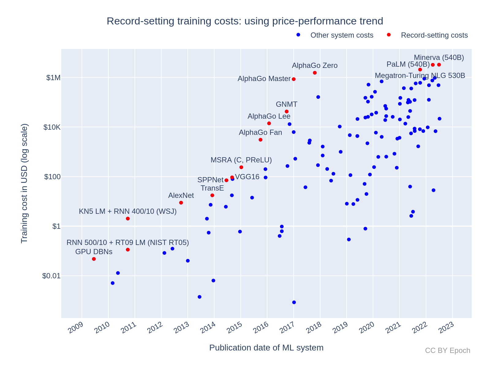
Figure 9: Training cost estimated using Method 1, with record-setting costs marked in red.
Looking at the most expensive training runs over time (plotted in red in Figure 9), the record-setting systems for cost are similar to the record-setting systems for training compute.58 It is notable that all of the AlphaGo systems (Fan, Lee, Master, Zero) were record-setting according to this estimation method. AlphaGo Master and AlphaGo Zero are particular outliers—AlphaGo Zero is 3.7 OOMs above the trendline mean. This cost record for AlphaGo Zero (estimated here as $1.5M) was not beaten until the language models Megatron-Turing NLG ($2.1M) and PaLM ($3.2M) about four years later. This is a much larger time period between records than any periods before AlphaGo Zero (which are about two years or less). AlphaGo Zero was also more anomalous in financial investment than Megatron-Turing NLG and PaLM. PaLM is only 1.7 OOMs above the mean by comparison, and many more systems costing between $100K and $4M occurred between 2019 and 2022. The most expensive system to train was Minerva in 2022, at an estimated $3.2M.
Method 2 dataset: GNMT stands out; Megatron-Turing NLG is top
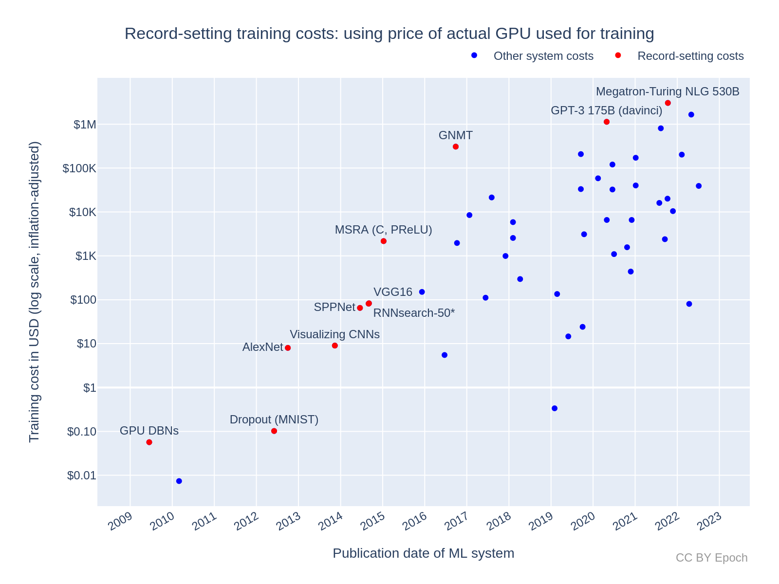
Figure 10: training cost estimated using Method 2, with record-setting costs marked in red.
When considering the most expensive training runs in the Method 2 dataset, an important caveat is that many of the systems in the full dataset (n=124) are missing. In particular, many of Google and DeepMind’s milestone systems in recent years are absent, because they were trained on Google TPUs rather than NVIDIA GPUs. These systems include AlphaGo and PaLM.
With that said, the character of record-setting training costs in the Method 2 dataset (shown in Figure 10) is similar to that of the Method 1 dataset. The most outlying cost record in this dataset is GNMT, which was published in September 2016. GNMT cost an estimated $300K, 3.1 orders of magnitude above the trend line. The next record was GPT-3 in May 2020, at $1.1M, or 2.1 OOM above the trend. The time period between these records, at about 3.5 years, is the largest time period between records in this dataset. The most expensive system in this sample is Megatron-Turing NLG in late 2021, at $3.0M, or 1.9 OOM above the trend. This is higher than the $2.1M estimate using Method 1.
Appendix F: Robustness of the regression results to different date ranges
Key takeaways:
- The mean growth rate predicted by Method 1 (roughly 0.5 OOMs/year) seems reasonably robust across different date ranges. The lowest mean out of four date ranges is 0.44, and the highest mean is 0.58. The confidence intervals on these growth rates mostly overlap.
- Method 2 is much less robust in this way. The lowest mean out of three date ranges is 0.35, the highest is 0.84, and the 90% confidence intervals of those two results do not overlap.
- I expect that obtaining a larger data sample for Method 2 would close most of this gap in robustness.
To check how robust the regression results are for the compute cost of final training runs of ML systems, I re-ran the regression on different date ranges. The results are listed in Table 4. I chose date ranges that seemed particularly meaningful (for reasons explained below), but it also seems reasonable to use random date ranges.
- For both Method 1 and Method 2, I used the following date ranges:
-
September 2015–2022: I chose this date range to coincide with the “Large Scale Era” in which all “Large Scale” systems occur, since that era is characterized by higher variance and arguably has a “Large Scale” trend occurring separately from the “Deep Learning” trend.59
-
2009–August 2015: similarly, I chose this date range to immediately precede the “Large Scale Era.”
-
- In addition, for Method 1 only, I used the date range of October 20th, 2017–2022. I chose this date range to exclude all AlphaGo systems (but it also excludes other systems that occurred in 2015–2017). All AlphaGo systems had record-setting costs (see Figure 9 in this section), and AlphaGo Master and AlphaGo Zero are particularly large outliers, so I expected the AlphaGo systems’ cost values to have a significant influence on the regression results.
- Note that the dataset for Method 2 coincidentally does not include any AlphaGo systems, because they were trained using Google TPUs, and I have only collected data on systems trained with NVIDIA GPUs.
| Estimation method | Period | Data | Growth rate (OOMs/year) |
|---|---|---|---|
| Method 1 (using average trend in hardware prices) | 2009– 2022 (i.e., the maximum period) |
All systems (n=124) | 0.51
90% CI: 0.45 to 0.57 |
| 2009– August 2015 |
All systems (n=23) | 0.55
90% CI: 0.34 to 0.75 |
|
| September 2015– 2022 |
All systems (n=101) | 0.44
90% CI: 0.27 to 0.61 |
|
| October 20th, 2017– 2022 |
All systems (n=83) | 0.58
90% CI: 0.35 to 0.80 |
|
| Method 2 (using actual hardware prices) | 2009– 2022 (i.e., the maximum period) |
All systems (n=48) | 0.44
90% CI: 0.34 to 0.52 |
| 2009– August 2015 |
All systems (n=9) | 0.84
90% CI: 0.61 to 1.14 |
|
| September 2015– 2022 |
All systems
(n=39) |
0.35
90% CI: 0.14 to 0.55 |
Table 4: growth rates of the compute cost of final training runs of ML systems, according to log-linear regressions on the cost data in different date ranges.
Other observations besides the key takeaway:
- Data in the period between September 2015 and October 2017 makes the estimated growth rate slower than it would be otherwise. Using a date range from September 2015 to 2022 results in a growth rate of 0.44, while moving the start date to October 2017 (after all AlphaGo systems were published) changes the growth rate to 0.58.
- Restricting to the September 2015–2022 date range increases the size of the confidence interval by a large amount (from 0.12 up to 0.34 for Method 1, and from 0.18 up to 0.41 for Method 2), despite a relatively small reduction in sample size. I think this is due to a higher variance of cost in that date range compared to the 2009–August 2015 date range, which can be seen visually in Figure 2 and Figure 4.
- While the growth rate for Method 2 in the date range of 2009–August 2015 is radically different to the other results, I put much less weight on it than the other results due to the very small sample size. The date range of September 2015–2022 gives a much closer result to the full date range (0.35 compared to 0.44).
Appendix G: Method 2 growth rate is due to the smaller sample of ML systems, but its estimates are ~2x higher than Method 1 on average
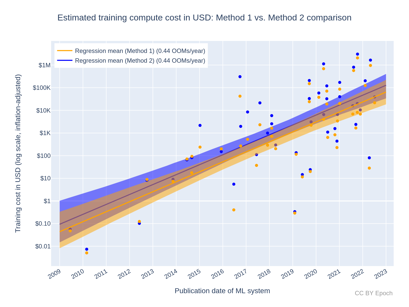
Figure 11: comparison of training cost estimates using the dataset of ML systems for which I obtained training hardware data: (a) in blue, the cost estimates and fitted trend using the price-performance of the actual GPU used to train the ML system, (b) in orange, the cost estimates and fitted trend using the price-performance value predicted by the trend line for GPU price-performance. See this Colab notebook cell for an interactive version of the plot with ML system labels.
Figure 11 illustrates how the growth rate found with Method 2 (0.44 OOMs/year) mostly depends on the smaller dataset of ML systems than on the use of discrete GPU price-performance data. This is because if we use Method 1 on this smaller dataset, the growth rate of the trend is the same. The similar growth rates suggest that, although Method 2 accounts for the delay between better GPUs being released and those GPUs being used in ML training runs, this delay is roughly constant on average in the dataset. The slope in the trend is the same, but the prediction is shifted by about seven months.60 Equivalently, the mean prediction for Method 2 is consistently about 2x higher than the Method 1 trendline.61
Appendix H: Comparison points for the cost estimates
Other cost estimates for PaLM and AlphaGo Zero seem too high, but my estimates are probably still too low
Below are three cost estimates from other sources, which are based on more system-specific estimation methods than I used:
- PaLM: $17M, $23.1M, and $9.2M. Compare this to the Method 1 estimate of $3.2M.62
- $17M: The estimation model was essentially the formula that I presented at the end of this section—multiplying training time in core-hours, the number of hardware cores, and the cloud compute price of that hardware.
- $23.1M: This is similar to my estimation model using training compute and hardware price-performance. However, here the cloud compute price is substituted for the (hardware_unit_price / hardware_replacement_time) formula that I used. This $/s value converts FLOP/s into FLOP/$.
- $9.2M: This is similar to the method for (a), but uses the cloud compute pricing of LambdaLabs and substitutes an NVIDIA A100 GPU for the TPU V4.
- AlphaGo Zero: $35 million. Compare this to the Method 1 estimate of $1.5M.
- The estimation model for the $35 million estimate was essentially the formula that I presented at the end of this section—multiplying training time, the number of hardware units, and the cloud compute price of that hardware.
- GPT-3: $4.6M. Compare this to the Method 2 estimate of $1.1M.
- The estimation method here was to calculate the hypothetical training time for a single NVIDIA V100 GPU, and multiply that training time by Lambda’s on-demand cloud compute price (per hour) for the V100 at the time. The differences to my estimate are in the assumed hardware utilization rate (my 35% vs. their 25%)63 and the hardware cost per hour (my $0.52 vs. their $1.50).64
There are strong reasons to believe that the above reference estimates are all at least 2 times larger than the true cost for system developers. This is because all of the estimates are based on prices for an end-consumer paying a cloud vendor for renting hardware on-demand by the hour. As of August 26, 2022, Google Cloud offers a 37% discount on TPU V4 prices for a one-year rental commitment, and a 55% discount on the on-demand price for a three-year rental commitment. Presumably, Google Cloud still makes a profit even when the 55% discount is applied. So for AI developers such as Google Research that use in-house computing clusters,65 the final training run cost would be at least 55% lower, and probably even lower than that. A 55% discount on the estimate for PaLM above that is most similar to my method ($23.1M) is $10.4M, which is much closer to my estimate of $3.2M but still far apart.
For AlphaGo Zero, the self-play data used for training was performed on TPU V1 chips, which were about 20x more expensive than one of the GPUs on Google Cloud at the time.66 The TPU compute costs dwarfed the GPU compute costs, according to the reference estimate. It is possible that DeepMind or Google paid a proportionately high premium to buy these TPUs. However, a Wired article from 2017 states “During the development of Zero, [DeepMind CEO Demis Hassabis] says the system was trained on hardware that cost the company as much as $35 million.”67 This is the same as the estimate of the training compute cost of AlphaGo Zero above, an estimate which was made in 2020—but that is probably somewhat of a coincidence. I interpret the article as saying that the cost to buy the TPUs was $35 million. In order to justify that cost, I expect that the TPUs were probably used for purposes other than AlphaGo Zero that used comparable amounts of compute to AlphaGo Zero itself (at least in total). So I think this evidence still points to the actual cost of training AlphaGo Zero being at least half of $35 million (i.e. ~$17 million). But that still makes it likely that for this particular system, my estimate is too low.
As another reference point, Cotra & Davidson estimated $2.8M for AlphaGo Zero, compared to my $1.5M. However, this is very correlated to my estimate because I used the same training compute estimate in FLOP as they did. Cotra & Davidson used a FLOP/$ estimate of about 1e17 in their calculation,68 whereas I used about 2e17.69
In another appendix, I explain my overall best guess that the true final training run compute cost of each ML system in my dataset is 2x higher (90% CI: 0.4x to 10x higher) than Method 2 estimates.
Forecasting TAI with biological anchors
One of the components of Cotra’s biological anchors model (henceforth “Bioanchors”) to forecast the arrival of transformative AI (TAI) is the “willingness to spend”—that is, the maximum amount of money that an actor is willing to spend on an AI training run at a given point in time. In simple terms, Cotra modeled willingness to spend as an exponential function of time, with an initial growth rate based on the long-term historical trend in computing hardware, which then flattens out to a growth rate dictated by the GDP of the richest country.70
One of the key parameters of the Bioanchors model is the compute cost for the most expensive training run at the start of the forecasting period (2025), in 2020 USD. Cotra’s best guess for this was $1 billion (i.e., $10^9). According to my data and estimates, the maximum compute spend in 2022 was for Minerva (540B), at $10^6.5 or roughly $3.5M. My aggregate estimate of the growth rate for all systems, at approximately 0.5 OOMs/year, predicts ~1.25 OOMs of growth relative to Minerva (published in June 2022) by the beginning of 2025. This means my model predicts a maximum spend of 10^(6.5 + 1.25) = $10^7.75 (~$60 million) by 2025. This is roughly one OOM lower than Cotra’s best guess.
Using the “Large-scale” trend value gives an even lower estimate of 10^(6.5 + [2.5 years * 0.24 OOMs/year]) = 10^7.1 (~$10 million) by 2025.71 Based on the analysis in another appendix, I think that my starting cost estimate for Minerva is most likely an underestimate. However, I think that the slower “large-scale” trend is more predictive of the longer-term limits on training cost than the trend that includes all systems. So let’s suppose my starting cost estimate were one OOM larger, at $10^7.5 (I think it’s more than 60% likely that the actual most expensive cost was lower than that72). Then my best guess would be $10^8.1 (~$130 million), which is still about one OOM lower than Cotra’s best guess.
Another key parameter in Cotra’s model of willingness to spend is the growth rate of spending on compute for the most expensive training run at the start of the forecasting period (2025), in years. According to Cotra’s best guess, this growth rate dominates until around 2035, when the limits of GDP growth dominate. Cotra’s best guess for this parameter is a doubling time of 2 years.73 This is close to the growth rate in GPU price-performance found in Trends in GPU price-performance (2.5 year doubling time), and corresponds to log10(2)/2 ~= 0.15 OOMs/year.
Again, my results here predict a growth rate of ~0.5 OOMs/year (or doubling time of ~0.63 years), which is much faster than Cotra’s best guess of 0.15 OOMs/year. Cotra did account for historical rapid growth in their reasoning, believing that this kind of growth would continue from 2020 to 2025, but then return to the longer-term historical growth rate that is similar to hardware price-performance.74 The finding that the growth rate in “large-scale” systems since 2016 is already slower,75 at 0.2 OOMs/year, suggests that the slowdown of growth in spending may be happening sooner than Cotra expected in 2020.
I don’t think my findings have any significant implications for the other two parameters of Cotra’s model of willingness to spend—namely, the maximum fraction of GDP that actors are willing to spend on computation, and the growth rate in GDP.
AI and Compute (CSET)
CSET’s “AI and Compute” (Lohn & Musser, 2022) uses a similar method to the one used here to combine the growth rate in training compute (in FLOP) with the growth rate in hardware price-performance (in FLOP/$) to forecast training compute costs in dollars. Lohn & Musser’s analysis is most sensitive to the compute growth rate, because the growth rate they used (a 3.4-month doubling time, equivalent to 1.1 OOMs/year)76 is much slower than the growth rate in FLOP/$ (with a doubling time of four years in their median estimate, equivalent to 0.08 OOMs/year).77 The resulting growth rate in training cost that they estimate is therefore 1.1 - 0.08 ~= 1.0 OOMs/year.78 This is roughly double my overall estimate of the historical growth rate of 0.49 OOMs/year from 2009–2022. So where their method projects +5 OOMs of growth in cost by 2027 (roughly matching the projected US GDP by that year), my method projects that amount of growth in twice the duration, i.e., by 2032. Using the more conservative growth rate of 0.2 OOMs/year found for large-scale systems, +5 OOMs would only be reached in 21 years (2043).79 The basic point still stands that recent growth in spending seems unsustainable over the next few decades, but I think that compute spending flattening out by 2027 vs. 2043 has quite different implications for AI timelines and AI governance.
Another discrepancy between this work and CSET’s “AI and Compute” is the estimate for the most expensive training run in 2022. As described in p.10 of their report, Lohn & Musser seem to project an estimated 3.4 month compute doubling time from 2018–2019 into 2021, to get a cost of $450 million.80 I think this estimate is too high for the actual cost.81 Given that the report was published in 2022, I find it too aggressive to assume a cost of $450 million in 2021, since that cost almost certainly was not incurred for the final training run of any known, published ML system. Based on my estimates and estimates in other work (see this section), I am 70% confident that the most expensive ML training run that occurred in 2021 cost at least one OOM lower (i.e., less than $45 million) in compute.
Appendix I: Overall best guess for the growth rate in training cost
In another appendix, I reviewed prior work that assessed and projected the compute cost to train ML systems, in comparison to my results. Building on that review, this appendix outlines the reasoning for my overall best-guess answer to the following question: which constant growth rate would result in the most accurate prediction of the final training run cost of a transformative ML system? Here, I’m assuming a model like Cotra (2020) where this growth rate is sustained up until it hits a limit due to gross world product growth. My independent impression for this growth rate is 0.3 OOMs/year (90% CI: 0.1 to 0.4 OOMs/year), while my all-things-considered view is 0.2 OOMs/year (90% CI: 0.1 to 0.3 OOMs/year). My reasoning is as follows:
-
Using the results in this report as a starting point, I created a mixture model of the “large-scale” growth rate (obtained via Method 1, since I considered the sample size for Method 2 to be too small) and the aggregate growth rate for “all systems.”82 These growth rates are reported in Table 3 and Table 2, respectively. The resulting aggregate growth rate was 0.39 OOMs/year (90% CI: 0.13 to 0.55 OOMs/year).
-
To check the plausibility of this initial result, I considered the potential ceiling to spending on final training runs, and when that ceiling will be reached based on the current growth rate.
-
For the ceiling on spending, I deferred to Cotra (2020): 1% of GDP of the richest country.83 However, my method is even simpler than Cotra’s method, as I just take 1% of the current approximate GDP of the United States as a constant ceiling.
-
United States GDP: ~20 trillion ~= 13.3 in log10 units84
-
1% of that = 13.3 - 2 = 11.3 in log10 units = $200 billion
- One reference point: Alphabet revenue was 257.6 billion USD in 2021 according to Wikipedia. So even today, this budget wouldn’t instantly wipe out Alphabet’s revenue. But it seems implausible for Alphabet to stake most of their revenue on a single ML system training run. So I think this ceiling is reasonable as an amount which is very plausible 10 years or more in the future, but not plausible today.
-
- I will use my predicted cost of Minerva (6.5 in log10 units) as the starting point, because my data suggests it is the most expensive system to date.
- The year in which that ceiling of spending is reached would therefore be 2023 + (11.3 - 6.5 OOMs) / (0.39 OOMs/year) ~= 2023 + 12 = 2035.
- Based on current private tech company revenue (e.g., Alphabet revenue was reportedly US$257.6 billion in 2021), and my very rough intuitive sense of what would be reasonable to spend on a single training run as AI capabilities improve and generate more revenue, I think it’s more than 10% likely that spending on compute to train a single ML system could reach $200 billion by 2035.
- But I don’t think this is more than 50% likely by 2035.
- So my best guess for the growth rate would have to be less than 0.4 OOMs/year.
- Cotra’s reasoning for spending growth slowing down after 2025 to a two-year doubling time (about 0.15 OOMs/year) also persuades me to choose a lower growth rate.
-
Lohn & Musser (2022) argued that recent growth in spending on compute leads to reaching an amount equal to US GDP before 2030, and that this is implausible.85 I treat the claim that it is implausible for spending to become comparable to US GDP as mostly independent of the disagreements that I outlined previously. So this claim persuades me to choose a lower growth rate.
- Based on an intuitive judgment of how to weigh the above evidence, I adjusted the initial growth rate of 0.39 OOMs/year (90% CI: 0.13 to 0.55 OOMs/year) down by 25%, to 0.29 OOMs/year (90% CI: 0.10 to 0.41 OOMs/year). Given the lack of precision in my method, I then rounded this to 0.3 OOMs/year (90% CI: 0.1 to 0.4 OOMs/year). This estimate is my independent impression.
- My all-things-considered view (as opposed to my independent impression) defers more strongly to Cotra (2020), adjusting my initial growth rate estimate down by 50% to 0.2 OOMs/year (90% CI: 0.1 to 0.3 OOMs/year). Again, this degree of adjustment is entirely based on my intuition of how much I ought to adjust, rather than a principled calculation.
-
Note that in contrast to the overall period between now and TAI, I expect that when measured on shorter timescales (e.g., 2–5 years), the growth rate in the cost to train large-scale systems will most likely reach higher than 0.3 OOMs/year at some point between now and when TAI is developed. This is because I expect the growth rate in AI investment will increase at some point when AI can demonstrably have a major impact on the economy.86 However, I think there is currently a lot of uncertainty about the trends of and the relationships between investment in AI, the allocation of spending in AI, and revenue generated by AI systems. Investigating those areas is therefore an important topic for future work.
Appendix J: Overall best guess for training cost
Neither of the two cost estimation methods used in this work directly represent my all-things-considered, best estimates of the true cost of compute for the final training run of ML systems. The estimates via these methods are informative, but they have strong simplifying assumptions that I expect to add bias and variance relative to the true values. In this appendix, I explain how I account for these limitations in a very rough way to obtain my overall best guess for training costs.
I believe that the cost estimates of Method 2 are more accurate than Method 1, because Method 2 uses prices for the specific hardware used to train each ML system. So I use Method 2 as my reference point for the best guess rather than Method 1. However, once I account for factors of overestimation and underestimation in Method 2, I find that these factors roughly cancel out, so the estimates of Method 2 happen to be similar to my best guess. Meanwhile, the estimates of Method 1 are roughly 2x lower than this best guess.
My independent impression is that the estimates of Method 2 are accurate on average—this is due to factors of overestimation and underestimation roughly canceling out, rather than directly choosing Method 2 as my best guess. However, because the estimates of Method 2 are much lower than estimates from other sources (see this section), my all-things-considered view is that the true final training run compute cost of each ML system in my dataset is 2x higher87 (90% CI: 0.4x to 10x higher)88 than Method 2 estimates.
Method 2
Overall best guess about how this method is inaccurate
Accounting for the potential sources of overestimation (0.46x factor) and underestimation (2x factor) in this method, the factors roughly cancel out. So my best-guess independent impression is that the estimates of Method 2 are roughly accurate on average. However, my 90% CI for that best guess is 0.2 to 5 times what Method 2 estimates (see this section). To be clear, I did not update my estimates of the error in order to make the factors cancel out. This was the result I obtained after estimating each source of error that I could think of, and I am surprised that the factors happened to roughly cancel out.
Sources of overestimation
- Overall: accounting only for the potential sources of overestimation listed below, the true value would be (1 - 0.39) * (1 - 0.25) ~= 0.46, i.e., 54% lower than my original estimate.
-
The actual hardware cost paid for the largest purchases of GPUs (e.g., cloud compute providers, or top AI labs that have their own data centers) would typically be less than publicly reported prices, because I expect that those buyers negotiate the price down for those purchases.89 There could also be unpublicized bulk discounts that are applied to hardware purchases but are not explicitly negotiated. Accounting for this, my intuitive guess is that the true price paid in the largest purchases of GPUs is half of the price value that I used in my estimates. But I also guess that this price reduction only applies to 77% of the ML systems in my dataset, based on how many systems had industry involvement.90 A 50% reduction in cost for 77% of cases is a ~39% reduction in cost on average. (+39% error)
- Hardware price for the same GPU model tends to decrease overall on long enough timescales, i.e., two to four years. (+16% error)
- Price fluctuates up and down. But based on the first plot in this article, over time intervals of two years, the price of most NVIDIA data center GPUs decreases. For all of the GPUs in that plot, the price of the GPU in 2022 is lower than the initial price (which goes as far back as 2012).
- Estimating this decrease on average
- Looking at the empirical timing of ML systems using NVIDIA V100 GPUs in Figure 7, its usage spans the past four years. Based on this, I assume that for a given GPU model, the ML systems in my dataset that were trained using that GPU model were published halfway through on average, i.e. two years after the release of the GPU model.
- If we assume that the trend in GPU price-performance not only implies that newer GPUs have higher FLOP/second per dollar, but also that older GPUs get cheaper at the same rate, then each existing GPU would be getting cheaper at a rate of half every 2.5 years.
- This implies that each existing GPU gets 2^(-2/2.5) ~= 57% as expensive one year after release, i.e. a decrease of 43%.
- As an alternative method, I looked at the actual change in NVIDIA GPU prices (for the PCI-Express versions of the GPU) in the first two years after release (again based on the first plot in this article):
- A100 decreased ~15%
- V100 increased ~20%
- P100 ~0% change
- K80 decreased ~20%
- K40 decreased ~15%
- K20 decreased ~10%
- Unweighted average: (-15 + 20 + 0 + -20 + -15 + -10) ~= 7% decrease
-
So empirical data suggests a smaller decrease than what is implied by the 2.5 year doubling time in price-performance (7% vs. 25% respectively). However, this is slightly biased by the chip shortage circa 2020, which increased the price of the V100 and A100 in 2020.91
- I will interpret this 7% decrease as a 7% overestimate, again assuming that for a given GPU model, the ML systems in my dataset that were trained using that GPU model were published two years after the release of the GPU model, on average.
- Taking the average of my 43% and 7% estimates above, I get a 25% decrease in hardware price. This alone would suggest that my cost estimates are too high by 25%.
Sources of underestimation
- Overall: accounting only for the potential sources of underestimation listed below, the true value would be (1 + 0.4) * (1 + 0.2) * (1 + 0.2) ~= 2.0, i.e., 100% higher than my original estimate.
- Some models may have been trained via compute provided by cloud compute vendors. Due to the profit margin of cloud compute vendors, the training cost in those cases would be higher.
- Setting the cloud compute profit margin to 67%,92 the underestimate would be a factor of 1/(1 - 0.67) ~= 3x. But I’d guess this is only for 20% of the ML systems. If 1 in every 5 systems have 3x the cost that I estimated, then the factor of increase in the average cost would be (4x1 normal systems + 1x3 cloud compute system) / (5 systems) = (4 + 3) / 5 = 1.4, i.e., a 40% increase. (-40% error)
- Neglecting the energy cost of running the hardware. (-20% error based on the GPT-3 example in another appendix.)
- Neglecting the cost of other hardware that makes up data centers (e.g., switches, interconnect cables). (-20% error. This is an intuitive guess, anchored to the energy cost error. I would be surprised if the cost of this is a much larger fraction than this—given the extremely advanced manufacturing required for modern GPUs, it seems like they ought to be a more expensive individual hardware component than everything else combined.)
Confidence interval based on factors that overall seem to add variance but not significant bias to the estimates
In what follows, I estimate 90% confidence intervals for the variables in the cost estimation formula for Method 2.93 I then combine those confidence intervals to get an overall 90% CI for my training cost estimates: 0.2x to 5.0x the central estimate. Note that these are subjective estimates. My choice of numbers was probably somewhat influenced by making the numbers round, rather than purely choosing my most precise best guess.
- Hardware price ($): 0.5x to 2.0x the central estimate
- Fluctuation over time due to market forces
- Variation by a factor of 1.5x seems typical—see Footnote 12 for observations
- To be more conservative than what those limited observations suggest, I chose a factor of 0.5x to 2x
- Fluctuation over time due to market forces
- Compute (in FLOP): 0.5x to 2.0x the central estimate
- I used the same factor of uncertainty as Sevilla et al. (2022, p.16), 0.5x to 2x.
- Hardware utilization rate (%): 10% to 60% (0.29x to 1.71x the central estimate)
- I chose a confidence interval for this based on the “About GPU utilization rates” box in the post Estimating Training Compute of Deep Learning Models, which cites 11 specific utilization rate estimates.
- Lower bound
- The lowest utilization rate reported in that section is 10%, but that number was reported by its original author as a “subjective estimate.”
- In figure 5 of (Patterson et al, 2021), the authors report GPU usage rates as low as 20% (25 divided by 125) for GPT-3. This is the second-lowest number in the several examples given in the post.
- Overall, it seems reasonable to choose 10% as my 5th percentile, to account for the possibility of rates less than 20% that were not reported.
- Upper bound
- I think that my uncertainty in the hardware utilization rate is better modeled as a normal distribution than a log-normal distribution, because it is a percentage and reported values seem to be fairly concentrated between 20% and 50%.
- So by the symmetry of the normal distribution, if the 5th percentile is 25 percentage points below the mean of 35%, then the 95th percentile should be 25 percentage points above, at 60%. This is roughly 1.71x my central estimate of 35%.
- As a check for this choice of 60%, the highest utilization rate achieved for an actual milestone ML system that is listed in the post is 56.5% for Google’s LaMDA model. So choosing 60% seems reasonable, but it may be too low as a 95th percentile.
- There are higher numbers listed (75% based on “experiments on different convolutional neural networks with single GPUs,” and “GSPMD reportedly yields rates as high as 62% at scale”), but I don’t find these numbers as plausible for most milestone ML systems in practice, because my impression (without checking precisely) is that the majority of milestone ML systems have been trained with multiple GPUs.
- Lower bound
- I chose a confidence interval for this based on the “About GPU utilization rates” box in the post Estimating Training Compute of Deep Learning Models, which cites 11 specific utilization rate estimates.
- Hardware replacement time: one to four years (0.5x to 2.0x the central estimate)
- Replacing hardware faster than one year of continuous use seems unreasonable given the cadence at which better hardware is released, and given the overhead cost of the replacement process. NVIDIA seems to release new data center GPUs roughly every two years based on the first plot in Morgan (2022). On the other hand, waiting longer than four years of continuous use to replace hardware also seems unreasonable, based on the timing of better data center GPUs being adopted in ML (see Figure 7). So my 90% CI for this is one to four years.
- The actual number I used for the estimates was two years, so the factor of uncertainty is 0.5x to 2x.
To estimate a confidence interval, I took the 5th and 95th percentile of 10,000 samples of training cost (expressed as a ratio of my central estimate, e.g. 0.5x).94 For each of those samples, I sampled a factor for each of the above variables from a log-normal distribution95 with the bounds specified above. I then multiplied and divided those factors according to my cost formula to get the final cost ratio for that sample. The resulting overall 90% CI in training cost was 0.2x to 5.0x the central estimate.
Method 1
Based on the comparison of estimates between Method 1 and Method 2 in another appendix, my best guess is that Method 1’s estimates are 2x lower on average than Method 2. So Method 1 is inaccurate in similar ways to Method 2, but it additionally underestimates cost by a factor of 2x on average.
Notes
-
These are “milestone” systems selected from the database Parameter, Compute and Data Trends in Machine Learning, using the same criteria as described in Sevilla et al. (2022, p.16): “All models in our dataset are mainly chosen from papers that meet a series of necessary criteria (has an explicit learning component, showcases experimental results, and advances the state-of-the-art) and at least one notability criterion (>1000 citations, historical importance, important SotA advance, or deployed in a notable context). For new models (from 2020 onward) it is harder to assess these criteria, so we fall back to a subjective selection. We refer to models meeting our selection criteria as milestone models.” ↩
-
This growth rate is about 0.2 OOM/year lower than the growth of training compute—measured in floating-point operations (FLOP)—for the same set of systems in the same time period. This is based on the 2010 – 2022 compute trend in FLOP for “all models” (n=98) in Sevilla et al. (2022, Table 3), at 0.7 OOMs/year. Roughly, my growth rate results from the growth rate in compute subtracted by the growth rate in GPU price-performance, estimated by Hobbhahn & Besiroglu (2022, Table 1) as 0.12 OOMs/year. ↩
-
These results are not my all-things-considered best estimates of what the growth rate will be from now on; rather, it is based on two estimation methods which combine training compute and GPU price-performance data to estimate costs historically. These methods seem informative but have strong simplifying assumptions. I explain my overall best guesses in point 3 of this summary, but those are based on more subjective reasoning. I base my cost estimates on reported hardware prices, which I believe are more accurate than on-demand cloud compute prices at estimating the true cost for the original developer.# This means my cost estimates are often one order of magnitude lower than other sources such as Heim (2022). ↩
-
This is the mean cost predicted by linear regression from the start to the end of the period. ↩
-
For these large-scale results, I dropped the precision to one significant figure based on an intuitive judgment given the lower sample size and wider confidence interval compared to the “All systems” samples. ↩
-
It turns out that this difference in growth rate to Method 1 is just due to the smaller dataset, even though the cost estimates differ significantly (roughly twice as large as those of Method 1 on average) (see this appendix for further explanation). ↩
-
I included this result for completeness, but given the very small sample size and large confidence interval on the growth rate, I do not recommend using it. ↩
-
The growth rates obtained via Method 1 and Method 2 were aggregated using a weighted mixture of normal distributions implemented in this Guesstimate model. Note that the results given by Guesstimate vary slightly each time the model is accessed due to randomness; the reported value is just one instance. ↩
-
The mixture method aggregates the growth rates rather than fitting a new regression to a dataset, so I did not obtain a mean prediction for this method. ↩
-
See the "Long-run growth" bullet in this section of Cotra (2020) titled "Willingness to spend on computation forecast". ↩
-
The adjustments are explained further in Appendix I and Appendix J. ↩
-
Sevilla et al. (2022) found that “before 2010 training compute grew in line with Moore’s law, doubling roughly every 20 months. Since the advent of Deep Learning in the early 2010s, the scaling of training compute has accelerated, doubling approximately every 6 months”. ↩
-
Several other significant costs are involved in developing and deploying ML systems, which I do not estimate. These costs include:
- Compute spent on experiments or failed training runs apart from the final training run
- Compute spent on training data collection and pre-processing
- Human labor to do research and implement experiments
- Maintenance of hardware and software infrastructure
- Operational support, including the hiring and management of personnel
- Compute and human labor spent on fine-tuning models for specific deployment applications
- Compute spent on model inference
-
As an extension for future work, one could use a non-linear model where soon after its release date, the hardware price is more expensive than the price closer to the end of the hardware’s life-span. Such a model could be based on empirical data on hardware price over time. ↩
-
This formula neglects energy costs associated with cooling the hardware. Based on the reasoning in this appendix, I think that total energy cost is generally small compared to hardware cost. ↩
-
For example, see Google Cloud GPU pricing: https://perma.cc/M5P3-MZF7 ↩
-
Parameter, Compute and Data Trends in Machine Learning. CC-BY Jaime Sevilla, Pablo Villalobos, Juan Felipe Cerón, Matthew Burtell, Lennart Heim, Amogh B. Nanjajjar, Anson Ho, Tamay Besiroglu, Marius Hobbhahn Jean-Stanislas Denain, and Owen Dudney. ↩
-
Since I estimate cost based on compute, my methods are similar to Sevilla et al. (2022). See this appendix for a list of differences in our methods. ↩
-
As one indication of the uncertainty, two different estimation methods were found to differ by up to a factor of 1.7x - see Estimating Training Compute of Deep Learning Models Appendix B. ↩
-
The 1.5x number is based on Morgan (2022): “…it is important to remember that due to shortages, sometimes the prevailing price is higher than when the devices were first announced and orders were coming in. For instance, when the [NVIDIA] Ampere lineup came out, The 40 GB SXM4 version for the A100 had a street price at several OEM vendors of $10,000, but due to heavy demand and product shortages, the price rose to $15,000 pretty quickly. Ditto for the 80 GB version of this card that came out in late 2020, which was selling for around $12,000 at the OEMs, and then quickly spiked to $17,500.” 15,000 / 10,000 = 1.5, and 17,500 / 12,000 ~= 1.5. ↩
-
This and the utilization rate estimate are the same as Ajeya Cotra used in the work “Forecasting TAI with biological anchors.” See Grokking “Forecasting TAI with biological anchors” for a summary, and in particular, this cell titled “Convert from LINPACK FLOP/s to total FLOP in training run” in this Colab notebook analyzing compute price trends. ↩
-
Based on Estimating Training Compute of Deep Learning Models recommending “30% for Large Language Models and 40% for other models.” I used the average of 0.3 and 0.4 given that my dataset includes Large Language Models and other models. The 0.35 value may be too low given that Large Language Models seem to make up a minority of the systems in the dataset. ↩
-
Scaling Laws for Neural Language Models provides evidence of this relationship in the language domain—empirically, the loss of a language model on the validation dataset improves as training compute scales, according to a power law. ↩
-
Compute Trends Across Three Eras of Machine Learning also initially used visual inspection to decide outliers—see p.16: “[W]e first decided by visual inspection which papers to mark as outliers and then chose the [Z-score] thresholds accordingly to automatically select them.” ↩
-
There is a slight discrepancy here which may be due to rounding. Starting with the doubling time of 5.6 months in Sevilla et al. (2022, Table 3), equivalent to log10(2) / (5.6/12) = 0.65 OOMs/year, the growth rate would be 0.65 - 0.12 = 0.53 OOMs/year. That number seems similar enough to the result of 0.51 OOMs/year here to be explained by the differences in which data are included—see this appendix for more information about differences to Sevilla et al. (2022). ↩
-
See the section “Affordability of compute” in this summary. Cotra’s predicted growth in spending after 2025 has a 2-year doubling time, equivalent to 0.15 OOMs/year. ↩
-
For these calculations, I used the trend values with higher precision before rounding: 0.25 OOMs/year (90% CI: 0.16 to 0.34) ↩
-
See this appendix for further explanation ↩
-
The growth rates obtained via Method 1 and Method 2 were aggregated using a weighted mixture of normal distributions, implemented in this Guesstimate model. ↩
-
See this Guesstimate model. The predictions for Method 1 and Method 2 were combined in the same manner as the growth rates. ↩
-
See the "Long-run growth" bullet in this section of Cotra (2020) titled "Willingness to spend on computation forecast". ↩
-
Source: https://data.worldbank.org/indicator/NY.GDP.MKTP.CD?locations=US ↩
-
I estimated this cost in this section of Appendix H: $3.27M * 10^(2.5 years * 0.5 OOMs/year) ~= $60M. ↩
-
These adjustments are explained in Appendix I and Appendix J. ↩
-
See this Guesstimate model for the calculations. To calculate the 90% CI in the year, I just substituted the lower and upper bound of the growth rate into the model, and then took the upper bound and lower bound of the resulting year estimate (respectively). I resorted to this because I got nonsensical results when I used the original distribution that I calculated for the growth rate (e.g. predictions of 100 years). This means that the 90% CIs in the year may be wider than optimal. ↩
-
Thanks to Lennart Heim for suggesting some of these ideas. ↩
-
One indication of the profit margin is that discounts of 37%–65% (relative to on-demand prices) are offered by Google Cloud for longer rental commitments. See GPU pricing on Google Cloud in 2022. ↩
-
See Table 4 (p.6) of Patterson et al. (2021) ↩
-
See Patterson et al. (2021)—the 11th row of Table 4, and the formula in section 2.5 (p.5), as well as section 2.3 (p.4). ↩
-
CC-BY Jaime Sevilla, Pablo Villalobos, Juan Felipe Cerón, Matthew Burtell, Lennart Heim, Amogh B. Nanjajjar, Anson Ho, Tamay Besiroglu, Marius Hobbhahn and Jean-Stanislas Denain. ↩
-
Milestone systems are defined in Compute Trends Across Three Eras of Machine Learning. On p.16: “All models in our dataset are mainly chosen from papers that meet a series of necessary criteria (has an explicit learning component, showcases experimental results, and advances the state-of-the-art) and at least one notability criterion (>1000 citations, historical importance, important SotA advance, or deployed in a notable context). For new models (from 2020 onward) it is harder to assess these criteria, so we fall back to a subjective selection. We refer to models meeting our selection criteria as milestone models.” ↩
-
Based on the “Deep Learning Trend” beginning in 2010 in Compute Trends Across Three Eras of Machine Learning ↩
-
This is as far as I could tell, from searching the publication for relevant keywords for about two minutes. My keywords were “GPU,” “TPU,” “CPU,” “NVIDIA,” “processor,” “Intel,” and “AMD.” For some publications where I suspected certain hardware might have been used, I searched terms such as “V100” (which refers to NVIDIA Tesla V100). Some publications only mentioned terms like this without mentioning any other keywords. Due to time constraints, for the last 30 systems in the dataset I did not search the publication because it either (a) was from Google (which would likely use TPUs that I didn’t have data on), (b) the system was from the Chinese sphere (so it is less likely to use hardware I have data on), (c) the system was not as notable (e.g., the GPT-Neo language model, which is much less powerful than contemporary language models like GPT-3). ↩
-
Some systems have missing data, so the number of systems could be higher than 25. ↩
-
Data on each hardware unit price often came from multiple sources. NVIDIA does not release suggested retail pricing for data center GPUs, so the price information I have for NVIDIA data center GPUs comes from reports in press releases, news articles, and expert estimates, e.g., Morgan (2022). I applied logical rules to select which data source to use case-by-case, rather than average the values from multiple sources, because the sources usually had similar values. To see how I selected which data source to use, check the formulas in the “Real price (2020 USD) - merged” column in the database. ↩
-
See this cell of the accompanying Colab notebook for the calculation of price-performance. ↩
-
To be precise, when these factors were present, the bounds of the 90% CI for the regression on “all systems” changed by 0.01 at most, but that could have been merely due to random variation in the bootstrap sample rather than the presence of the factors. ↩
-
See p.16 of Sevilla et al. (2022) for how the low-compute outliers were excluded: “Throughout the article, we have excluded low-compute outliers from the dataset. To do so, we compute the log training compute Z-score of each model with respect to other models whose publication date is within 1.5 years. We exclude models whose Z-score is 2 standard deviations below the mean. This criteria results in the exclusion of 5 models out of 123 between 1952 and 2022. The models excluded this way are often from relatively novel domains, such as poker, Hanabi, and hide and seek.” ↩
-
See Figure 5 on p.18 of Sevilla et al. (2022). ↩
-
See this Colab notebook cell for the calculation. ↩
-
Price information is not included with datasheets, e.g., the NVIDIA A100. See also Morgan (2022): “Nvidia does not release suggested retail pricing on its GPU accelerators in the datacenter, which is a bad practice for any IT supplier because it gives neither a floor for products in short supply, and above which demand price premiums are added, or a ceiling for parts from which resellers and system integrators can discount from and still make some kind of margin over what Nvidia is actually charging them for the parts.” ↩
-
This is my understanding from talking to a few experts and reading some machine learning papers about training the largest neural networks to date (e.g., Google’s PaLM system from 2022). Sid Black, who was the leading contributor to developing the GPT-NeoX-20B language model, told me in conversation (paraphrasing) that “Large language model training is bottlenecked by interconnect. If you don’t set up the software stack properly, it’s really slow.” In the paper for PaLM (on p.8), it says “An interesting aspect of two-way pod-level data parallelism is the challenge of achieving high training throughput for cross-pod gradient transfers at the scale of 6144 TPU v4 chips attached to a total of 1536 hosts across two pods.” (This quote is heavy on jargon, but my understanding is that “cross-pod gradient transfers” involve transferring data between hardware units in different “pods,” which are groups of hardware units.) ↩
-
See Figure 5, p.18 of Sevilla et al. (2022). This is not surprising given that Method 1 just divides the training compute by the value of the trendline in GPU price-performance. But hypothetically, if training compute had grown at a slower rate than it actually did, we might have seen later systems set a compute record but not a cost record. ↩
-
The existence of a separate category of “Large Scale” systems is argued in Sevilla et al. (2022, p.22) ↩
-
See this Colab notebook cell for the calculation. ↩
-
Calculation: (7 months / 12 months per year) * 0.44 OOMs/year ~= 0.26 OOMs = 10^0.26 ~= 2. ↩
-
I quote Method 1 estimates for PaLM and AlphaGo Zero because, although I believe Method 2 is more accurate on average, I did not have data for PaLM and AlphaGo Zero to use in Method 2. ↩
-
Footnote 6 of the post states “We double V100’s theoretical 14 TFLOPS of FP32 to get its theoretical 28 TFLOPS of FP16.” This number is very close to the actual number of 25 TFLOPS reported by Patterson et al. (2021, Figure 5) (on behalf of GPT-3’s developer, OpenAI). The theoretical peak performance listed for the V100 (PCIe version) by NVIDIA is 112 TFLOPS, so 28 TFLOPS corresponds to a utilization rate of 25%. In contrast, I assumed a utilization rate of 35% for all systems. ↩
-
I used a price of $9,029.66 (for one NVIDIA V100 GPU, inflation-adjusted), amortized over two years, which results in $9029.66 / (2 years * 365 days/year * 24 hours/day) ~= $0.52 / hour. Footnote 1 in the LambdaLabs post specifies a price of $1.50/hour. ↩
-
See PaLM paper, p.66: “We trained PaLM 540B in Google’s Oklahoma datacenter…” ↩
-
See the table in Footnotes in the post. TPU is $6.50/hour while GPU is $0.31/hour. The table says the GPU is “best,” but I’m not sure if this means it is the highest performance GPU available, or the cheapest GPU available. ↩
-
I find this source relatively untrustworthy because it does not provide a direct source for the information, but I still give it significant credence. ↩
-
This cell note says “Paul estimated 1e17 operations per dollar for pure compute used highly efficiently; I’m assuming 1e16 here to account for staff costs, failed experiments not included in the paper, inefficiency, etc.” But the number in the spreadsheet calculation is actually 1.2e17, so I’m not sure whether this is a typo or the note is not actually relevant anymore. If the assumption of one order-of-magnitude lower is right, then this is another reason my estimate differs: I’m excluding staff costs and failed experiments from my definition of “training compute cost.” ↩
-
The peak price-performance trend in Figure 7 is at about 1e10 FLOP/s per $ in 2017. 1e10 FLOP/s per $ * 35% utilization * (2 * 365 * 24 * 60 * 60 seconds) = 2.2e17 FLOP/$. ↩
-
See the section Willingness to spend on computation forecast in the draft report ↩
-
For this calculation, I’m using the more precise growth rate of 0.24 OOMs/year rather than the rounded final result of 0.2 OOMs/year. ↩
-
I will explain why I find more than 7.5 OOMs (~$32M) unlikely. Most of the compute to produce Minerva was used to train PaLM first—Minerva was trained with an additional 8% of PaLM’s compute in FLOP (see the “Training compute (FLOPs)” column for “Minerva (540B)” in the Parameter, Compute and Data Trends in Machine Learning dataset). This blog post by Lennart Heim estimated PaLM’s training cost using cloud computing (assuming you are not Google) at between $9M and $23M. Increasing that by 8% would raise the cost to about $10M to $25M. But it would cost less for Google because they used their own hardware (the PaLM paper states on p.66 “We trained PaLM 540B in Google’s Oklahoma datacenter”), so they don’t have to pay the profit margin of clouding computing from another vendor. For these reasons, I think it’s more than 90% likely that the actual cost of compute to train Minerva was less than the value of $32M that I use here. Furthermore, I think it’s more than 70% likely that Minerva was actually the most expensive training run in 2022 (including training runs that haven’t been publicized yet—I assume Cotra was also including those). This leads to my stated overall probability bound of 0.9 * 0.7 = 0.63 ~= 60%. ↩
-
In the section Willingness to spend on computation forecast of the draft report, Cotra writes: “I made the assumption that [the growth] would slow to a 2 year doubling time, reaching $100B by 2040.” Cell B7 in Cotra’s “best guess” calculation spreadsheet currently lists a doubling time of 2.5 years, but this may have been a later update. I am assuming that the report is the source of truth for Cotra’s best-guess estimates in 2020, rather than the spreadsheet. ↩
-
In the section Willingness to spend on computation forecast of the draft report, Cotra writes “Beyond ~$1B training runs, I expect that raising money and justifying further spending would become noticeably more difficult for even very well-resourced labs, meaning that growth would slow after 2025.” ↩
-
Note that this is not exactly a novel result. Compute Trends Across Three Eras of Machine Learning already noted this slowed growth in the training compute (in FLOP) of large-scale systems. The dollar cost of that training compute has similar characteristics because the trend in FLOP/$ is relatively reliable. ↩
-
This growth rate was sourced from OpenAI’s “AI and Compute”. I confirmed with the authors via email that this is the growth rate that was used for the cost estimates and projections. ↩
-
See Figure 2 (p.13) of their report. ↩
-
This subtraction of the growth rates corresponds to FLOP being divided by FLOP/$ in log-space to get the cost in $. ↩
-
I used the more precise estimate of 0.24 OOMs/year in this calculation, even though I don’t trust the value to that level of precision: 5 OOMs / 0.24 OOMs/year = 21 years. ↩
-
On p.10: “By the end of 2021, the trendline predicted several more doublings, for an anticipated model of just over one million petaFLOPS-days. Training such a model at Google Cloud’s current prices would cost over $450 million.” It is evident that they use this cost as the start of the projection in Figure 2 of their paper (on p.13), since the line starts roughly halfway between 10^8 and 10^9. ↩
-
The authors explained to me via email that this estimate was intended moreso to make the point that recent historical growth in compute is unsustainable (because that conclusion isn’t particularly sensitive to the choice of initial cost), rather than to be an accurate estimate of the highest cost in 2021. ↩
-
The mixture model was a weighted mixture of normal distributions, implemented in this Guesstimate model. ↩
-
See the section Willingness to spend on computation forecast in the draft report ↩
-
The answer returned by the Google search for “united states gross domestic product” is 23.32 trillion USD for 2021. ↩
-
On p.12–13: “Figure 2 shows that if we assume that compute per dollar is likely to double roughly every four years (solid line), or even every two years (lower bound of shaded region), the compute trendline [quickly] becomes unsustainable before the end of the decade.” Figure 2 shows extrapolated training compute costs equalling US GDP by about 2027. ↩
-
I’m uncertain how to measure “major impact on the economy,” but for illustration, automating 1% of all current human-occupied goods-and-services jobs plausibly seems like enough to increase the growth rate in spending on training runs. ↩
-
The 2x factor is based on the following reasoning. In this section I said “A 55% discount on the estimate for PaLM [that] is most similar to my method ($23.1M) is $10.4M, which is much closer to my [Method 1] estimate of $3.2M but still far apart.” If I defer somewhat to the reasoning behind the external PaLM estimate, I think the value after a 55% discount is applied is the most accurate value that I have readily available. However, I also believe the Method 1 estimate is 2x too low as mentioned previously. So as a very rough calculation, the ratio compared to Method 2 would be 10.4M / (2 * 3.2M) = 1.625. I round this up to 2 given the imprecision of my calculations. ↩
-
The 90% CI was obtained by multiplying the bound of the 90% CI derived in this section by 2. Note that this interval is reflective of the variation in how much any given ML system in my dataset cost, rather than my uncertainty in the average cost of all the ML systems. ↩
-
See the appendix on NVIDIA GPU price-performance for my reasoning ↩
-
The article says: “…when the Ampere lineup came out, The 40 GB SXM4 version for the A100 had a street price at several OEM vendors of $10,000, but due to heavy demand and product shortages, the price rose to $15,000 pretty quickly.” I’m assuming that the V100 price increased in 2020 for a similar reason. ↩
-
As of August 26, 2022, Google Cloud offers a 55% discount on the on-demand TPU V4 price for a three-year rental commitment. Presumably, Google Cloud still makes a profit even when the 55% discount is applied. So I increased from 55% to 67%, mostly because I don’t think the profit margin would be drastically larger, but partly to use a convenient number (roughly two thirds). ↩
-
The formula is cost = compute / ((peak_hardware_throughput / hardware_price) * hardware_replacement_time * hardware_utilization_rate) ↩
-
The exception was the hardware utilization rate, which was sampled from a normal distribution. ↩
About the authors

Related posts