Estimating Training Compute of Deep Learning Models
We describe two approaches for estimating the training compute of Deep Learning systems, by counting operations and looking at GPU time.
Published
Resources
ML Models trained on more compute have better performance and more advanced capabilities (see e.g. Kaplan et al., 2020 or Hoffman et al., 2022). Due to this, estimating and reporting compute usage is crucial to enable accurate comparisons between ML models.
Compute usage is commonly measured as the number of floating point operations (FLOP) required to train the final version of the system. To estimate this we can resort to two strategies: a) using information about the architecture and amount of training data, or b) using information about the hardware used and training time.
Below we provide two calculators that illustrate these methods.
Do you see a mistake or do you want to submit missing information about hardware specs? Fill this form and we will look into it.
Introduction
In this article we will explain (with examples) how to estimate the amount of compute used to train an AI system. We will explain two procedures, one based on the architecture of the network and number of training batches processed; and another based on the hardware setup and amount of training time.
This is largely based on AI and Compute, where the authors use these two methods to estimate the training compute of several milestone AI systems. We explain the methods in more detail.
Our final goal is to produce an estimate in terms of the number of floating point operations (FLOP) used to train the system. Other units exist - we discuss two other popular units in the table below.
|
Multadds / FMAs Some authors measure the number of multiplications-and-additions (multadds) that happen during training. Often those make up the bulk of the computation, and since one multadd is two FLOP we can often estimate FLOP in terms of multadds by multiplying by 2. Confusingly, some profilers consider a multadd as a single FLOP, since they are usually implemented as the single instruction Fused Multiply-Add (FMA) in the hardware. Since peak performance numbers of GPU specs usually consider a FMA as 2 FLOP1 we opt for that convention as well. |
Petaflops-day Another popular option is measuring in terms of petaflops-day, which is equivalent to the number of floating point operations that can be done by a machine operating at a speed of one petaFLOP per second in a day; that is, 1e20 FLOP. PetaFLOP-day levels of training compute for ML models were first reported around ~2016, so this unit makes more sense when working with models from that date onwards. |
Method 1: Counting operations in the model
The first method is quite straightforward, and can be summarized as:
\[ \text{training_compute} = (\text{ops_per_forward_pass} + \text{ops_per_backward_pass}) * \text{n_passes} \]
Where ops_per_forward_pass is the number of operations in a forward pass, ops_per_backward_pass is the number of operations in a backward pass and n_passes is the number of full passes (a full pass includes both the backward and forward pass) made during training.
n_passes is just equal to the product of the number of epochs and the number of examples:
\[ \text{n_passes} = \text{n_epochs} * \text{n_examples} \]
If the number of examples is not directly stated, it sometimes can be computed as the number of batches per epoch times the size of each batch n_examples = n_batches * batch_size.
The ratio of ops_per_backward_pass to the number of ops_per_forward_pass is relatively stable, so if we summarize it as fp_to_bp_ratio = ops_per_backward_pass / ops_per_forward_pass we end up with the formula:
\[ \text{training_compute} = \text{ops_per_forward_pass} * (1 + \text{fp_to_bp_ratio}) * \text{n_passes} \]
We estimate the value of fp_to_bp_ratio as 2:1 (see box below). The final formula is then:
\[ \text{training_compute} = \text{ops_per_forward_pass} * 3 * \text{n_epochs} * \text{n_examples} \]
This formula is a heuristic. Depending on the exact architecture and training details it can be off2. We have found it to be a reasonable approximation in practice3.
The ratio of backward pass operations to forward pass operations
Computing the backward pass requires for each layer to compute the gradient with respect to the weights and the error gradient of each neuron with respect to the layer input to backpropagate. Each of these operations requires compute roughly equal to the amount of operations in the forward pass of the layer. So the fp_to_bp_ratio is about 2:1.
The weight update can often be ignored, since it is common to use large batch sizes and update the weights using the accumulated gradient of many passes at once. This is also the case when weights are shared, as with CNNs.
A more precise relation can be found in the following table:
|
Most compute-intensive layers |
Compute-intensity of the weight update |
Backward-forward ratio |
|
First layer |
Large batch size OR compute-intensive convolutional layer |
1:1 |
|
First layer |
Small batch size AND no compute-intensive convolutional layers |
2:1 |
|
Other layers |
Large batch size OR compute-intensive convolutional layer |
|
|
Other layers |
Small batch size AND no compute-intensive convolutional layers |
3:1 |
You can read more about the backward-to-forward pass operation ratio in (Hobbhahn and Sevilla, 2021).
Forward pass compute and parameter counts of common layers
The remaining part is computing the number of operations per forward pass. Sometimes the authors are kind enough to provide this information in their papers. Most often, they do not, and we need to infer it from the architecture.
To help you do this, we have put together a table of common neural network layers, estimating their number of parameters and the number of floating point operations needed for a forward pass of the layer.
Note in many layers that the amount of FLOP in a forward pass is approximately equal to twice the amount of parameters. This suggests a reasonable alternative approximation of the number of operations if we already know the number of parameters and we know there is no parameter sharing. Reciprocally, this gives us a way to estimate the number of parameters from the amount of operations in a forward pass.
There are however many exceptions to this rule - for example CNNs have fewer parameters because of parameter sharing, and word embeddings make no operations.
A more precise heuristic is that the amount of operations in the forward pass is roughly twice the number of connections in the model. This is also satisfied by CNNs.
In addition, there are some software tools that can be used to automatically compute the number of parameters and the number of FLOP for the forward pass in an architecture. See appendix A for discussion on using these profilers.
|
Layer |
# parameters |
# floating point operations |
|
|---|---|---|---|
| Fully connected layer from $$N$$ neurons to $$M$$ neurons |
$$N \cdot M$$ + $$M$$ ≈ $$N \cdot M$$ |
$$2 \cdot N \cdot M$$ + $$M$$ + $$M$$ ≈ $$2 \cdot N \cdot M$$ |
|
|
WEIGHTS BIASES NONLINEARITIES |
|||
| CNN from a tensor of shape $$H \cdot W \cdot C$$ with $$D$$ filters of shape $$K \cdot K \cdot C$$, applied with stride S and padding P |
$$D \cdot K \cdot K \cdot C$$ + $$K \cdot K \cdot C$$ ≈ $$D \cdot K \cdot K \cdot C$$ |
$$2 \cdot K \cdot K \cdot C \cdot D \cdot H’ \cdot W’ $$ + $$H’ \cdot W’ \cdot D$$ + $$H’ \cdot W’ \cdot D$$ ≈ $$2 \cdot K^2 \cdot C \cdot H \cdot W \cdot D/S^2$$ |
where $$H’=(H-K+2P+1)/S$$ $$W’=(W-K+2P+1)/S$$ |
|
WEIGHTS BIASES NONLINEARITIES |
|||
| Transpose CNN from a tensor of shape $$H \cdot W \cdot C$$ with $$D$$ filters of shape $$K \cdot K \cdot C$$, applied with stride $$S$$ and padding $$P$$ |
$$D \cdot K \cdot K \cdot C$$ + $$K \cdot K \cdot C$$ ≈ $$D \cdot K \cdot K \cdot C$$ |
$$2 \cdot D \cdot H \cdot W \cdot C \cdot K \cdot K \cdot C$$ + $$D \cdot H \cdot W \cdot C$$ + $$W’ \cdot H’$$ ≈ $$2 \cdot D \cdot H \cdot W \cdot C \cdot K \cdot K \cdot C$$ |
where $$H’=S \cdot (H-1)+K-2 \cdot P$$ $$W’=S \cdot (W-1)+K-2 \cdot P$$ |
|
WEIGHTS BIASES NONLINEARITIES |
|||
| RNN with bias vectors taking an input of size $$N$$ and producing an output of size $$M$$ |
$$(N+M) \cdot M$$ + $$M$$ ≈ $$(N+M) \cdot M$$ |
$$2 \cdot (N+M) \cdot M$$ + $$M$$ + $$M$$ ≈ $$2 \cdot (N+M) \cdot M$$ |
|
|
WEIGHTS BIASES NONLINEARITIES |
|||
| Fully gated GRU with bias vectors taking an input of size $$N$$ and producing an output of size $$M$$ |
$$(N+M) \cdot M+M$$ + $$(N+M) \cdot M+M$$ + $$(N+M) \cdot M+M$$ ≈ $$3 \cdot (N+M) \cdot M$$ |
$$3 \cdot$$ [ $$2 \cdot (N+M) \cdot M$$ + $$M$$ + $$M$$ ] + $$5 \cdot M$$ ≈ $$3 \cdot 2 \cdot (N+M) \cdot M$$ |
|
|
UPDATE GATE RESET GATE CANDIDATE WEIGHTS BIASES NONLINEARITIES GATE COMBINATION |
|||
| LSTM with bias vectors taking an input of size $$N$$ and producing an output of size $$M$$ |
$$(N+M) \cdot M+M$$ + $$(N+M) \cdot M+M$$ + $$(N+M) \cdot M+M$$ + $$(N+M) \cdot M+M$$ ≈ $$4 \cdot (N+M) \cdot M$$ |
$$4 \cdot$$ [ $$ 2 \cdot (N+M) \cdot M$$ + $$M$$ + $$M$$ ] + $$5 \cdot M$$ ≈ $$4 \cdot 2 \cdot (N+M) \cdot M$$ |
|
|
FORGET GATE INPUT GATE CANDIDATE OUTPUT GATE WEIGHTS BIASES NONLINEARITIES GATE COMBINATION |
|||
| Word Embedding for vocabulary size $$V$$ and embedding dimension $$W$$ |
$$W \cdot V$$ |
0 |
|
| Self attention layer with sequence length $$L$$, inputs of size $$W$$, key of size $$D$$ and output of size $$N$$ |
$$W \cdot D+D$$ + $$W \cdot D+D$$ + $$W \cdot N+N$$ ≈ $$W \cdot (2 \cdot D+N)$$ |
$$(2 \cdot W \cdot D+2 \cdot D)$$ + $$(2 \cdot W \cdot D+2 \cdot D)$$ + $$(2 \cdot W \cdot N+2 \cdot N)$$ + $$L \cdot (2 \cdot D+1)$$ + $$L$$ + $$2 \cdot L \cdot N$$ ≈ $$2 \cdot W \cdot (2 \cdot D+N)+2 \cdot L \cdot (D+N)$$ |
|
|
QUERY KEY VALUE ATTENTION SOFTMAX OUTPUT |
|||
| Multi-headed attention layer with sequence length $$L$$, inputs of size $$W$$, key of size $$D$$, head output of size $$N$$, output of size $$M$$ and $$H$$ attention heads |
$$H \cdot$$ ($$W \cdot D+D$$ + $$W \cdot D+D$$ + $$W \cdot N+N$$)+$$(H \cdot N \cdot M+M)$$≈ $$H \cdot (W \cdot (2 \cdot D+N)+N \cdot M)$$ |
$$H \cdot$$ ($$(2 \cdot W \cdot D+2 \cdot D)$$ + $$(2 \cdot W \cdot D+2 \cdot D)$$ + $$(2 \cdot W \cdot N+2 \cdot N)$$ + $$L \cdot (2 \cdot D+1)$$ + L + $$2 \cdot L \cdot N$$)+$$(2 \cdot H \cdot N \cdot M+M+M)$$ ≈ $$2 \cdot H \cdot (W \cdot (2 \cdot D+N)+L \cdot (D+N)+N \cdot M)$$ |
|
|
QUERY KEY VALUE ATTENTION SOFTMAX OUTPUT MULTIATTENTION |
|||
Table 1: Parameter count and number of operations for some common neural network layers4.
Example: CNN-LSTM-FCN model
For example, suppose that we have a CNN-LSTM-FCN architecture such that:
- The input is a sequence of images of shape [400x400x5].
- The average length of each input sequence is 20 images.
- The CNN has 16 filters of shape 5x5x5 and is applied with stride 2 and padding 2
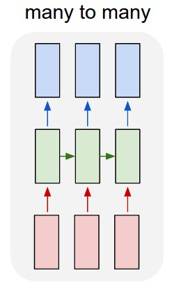
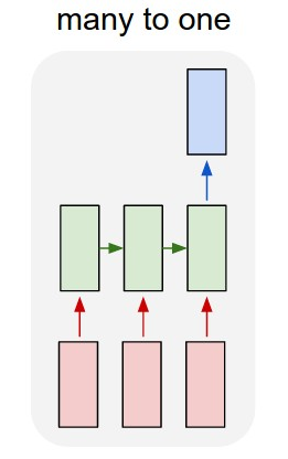
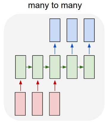
- The LSTM is a many-to-one layer with 256 output units and bias vectors
- The fully connected layer has 10 output units
- The training process takes 10 epochs, where each epoch consists of 100 batches of size 128 sequences each.
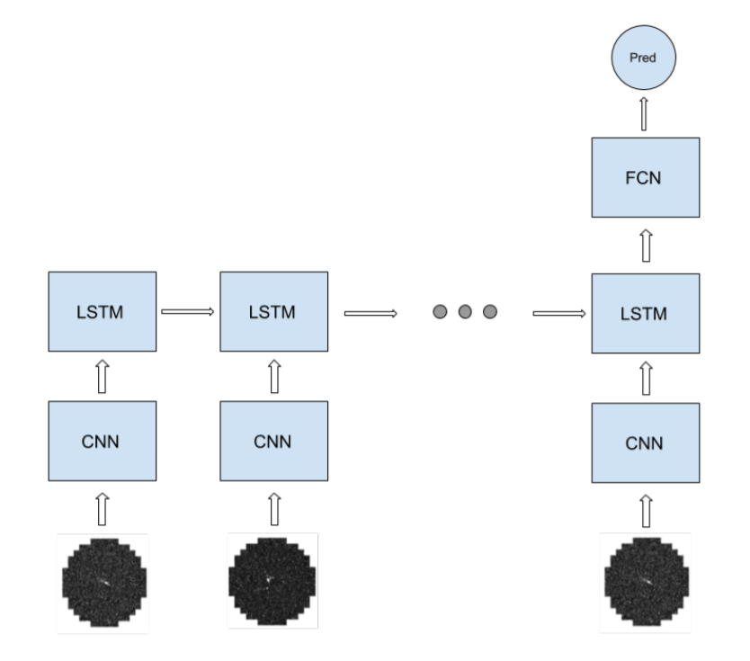
Figure 1: Diagram of the many-to-one CNN-LSTM-FCN from the example. Source.
Then we have that the recurrent part is the CNN and LSTM, and the FC is the non recurrent part of the network.
The CNN takes a 400*400*5 input and produces an output of width and height H’=W’=(W−K+2P)/S]+1=[(400−5+2*2+1)/2]=200 and 16 channels. In total, the forward pass of the CNN takes about 2*H2*W2*C*D/S2 = 2*4004*5*16/22 =1.024e12 FLOP.
Before feeding the input into the LSTM the output of the CNN is rearranged into a 200*200*16=640000 unit input. Then the amount of operations per token in the sequence of the LSTM is about 4*2*(N+M)*M=4*2*(640000+256)*256~=4*2*640000*256=1.310e9 FLOP. Finally, the FC layer takes about 2*N*M=2*256*10=5120 FLOP.
The non-recurrent part of the network is very small compared to the recurrent part, so we can approximate the number of total operations as
training_compute ~= ops_per_forward_pass_recurrent * 3 * n_epochs * n_batches * batch_size * avg_tokens_per_sequence ~= 1.024e12 FLOP * 3 * 10 * 100 * 128 * 20 = 7.86432e+18 FLOP.
When the architecture is too complex or we lack details of some of the layers we may want to use a method based on estimating the amount of operations from the amount of training time and the hardware used for training. We will cover that in the next section.
Example: Transformer
Let’s take a look at the Transformer architecture in Attention is all you need.
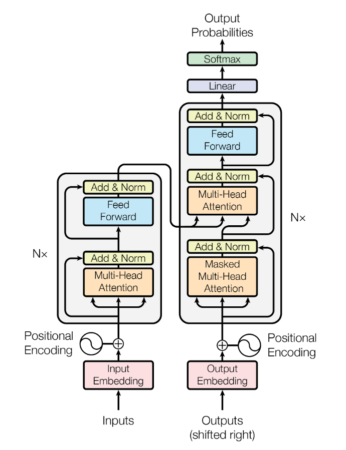
Figure 2: Diagram of the example Transformer architecture. Source.
- The input is a sequence of tokens, with an average length of 20 and a vocabulary size of 30,000.
- Each token is embedded and represented as a vector of size 1024.
- There are six encoder and decoder layers.
- Each encoder-decoder pair has a total of 3 multi-headed attention (MHA) sublayers, and 2 fully connected (FCN) sublayers.
- At the end there is a final linear layer and a softmax.
Each MHA sublayer has the following parameters:
- Input size W=64
- Head output size N=64
- Key size D=64
- Number of heads H=16
- Final output size M=1024
So the FLOP per token for a single MHA sublayer are 2*H*(W*(2*D+N)+L*(D+N)+N*M) = 2*16*(64*(2*64+64)+20*(64+64)+64*1024) ~= 2.6e6. Each FCN sublayer has an input size of 1024, output size of 1024, and a single hidden layer with 4096 units. So the FLOP per token for each sublayer are 2*2*N*M = 4 * 1024 * 4096 = 1.7e7.
Without taking into account the Add & Norm sublayers (they are negligible), the whole encoder-decoder stack has a total per-token FLOP of 6 * (3 * 2.6e6 + 2 * 1.7e7) ~= 2.5e8. The FLOP per token of the final linear layer (matrix multiplication) are 2 * 1024 * 3e4 = 6.1e7. The final softmax is negligible too, so a single forward pass of a full sequence takes 2.5e8 + 6.1e7 = 3.1e8 FLOP per token.
The paper says they use batches of 25,000 tokens, and run the training for 300,000 steps. So the total training FLOP would be 2.5e4 * 3e5 * 3 * 3.1e9 = 6.97e18 FLOP.
Method 2: GPU time
Instead of a detailed understanding of the forward pass compute, we can also use the reported training time and GPU model performance to estimate the training compute.
GPU-days describe the accumulated number of days a single GPU has been used for the training. If the training lasted 5 days and a total of 4 GPUs were used, that equals 20 GPU-days.
This metric has the obvious downside that it does not account for the computing hardware used. 20 GPU-days today are equivalent to more FLOP than 20 GPU-days ten years ago5.
In this section we will see how to correct for this. The final estimate will be:
\[ \text{training time} \times \text{# of cores} \times \text{peak FLOP/s} \times \text{utilization rate} \]
Estimating the number of FLOP from the GPU time
Step 1: Reading the paper
Extract the following information from the paper/reference:
- Number of GPU-days
- The computing system/GPU used
- When in doubt, one could go for the most common system used in same year publications or the geometric average of FLOP/s of computing systems in the same year.
- The number representations used during the training run: FP32, FP16, BF16, INT8, etc.
- When in doubt, I’d recommend defaulting to FP32, as this is the default option in most frameworks. However, in recent years FP16 has become more prominent.
Which number representation is used?
When looking up specifications sheets of computation hardware, you usually find the computational performance divided into different brackets based on the number representation, such as FP32, FP32, FP16, bfloat16, int16, or int8. This leads to the question: which performance metric should you pick?
Ideally you find the number representation used in the training process in the paper. Otherwise, we would recommend to rely on two heuristics:
1. In which years was the model trained?
Depending on the year trained and the framework used, the framework might have taken care of optimizing the training process by using the superior FP16. Starting in mid 2020, PyTorch does this automatically with supported hardware.
Work earlier than 2019 rarely used FP16, we’d suggest to default to FP32.
2. Who trained the model and how big is it?
Big models require more computational resources to train which leads to higher costs. This incentives to optimize the deployment. However, this optimization is not trivial. Given the high costs and non-trivial optimizations, we have seen big models usually emerging from corporate actors. They have dedicated ML engineers which can help with the deployment.
Consequently, for big models from corporations, we’d also default to use the number representations with the best computational performance (FP16 or bfloat16).
Anecdotally, we asked a couple of PhD students and most of them did not actively try to optimize their training run. Their answer was along the lines of “I press the train button and wait”. Therefore, we’d suggest referring to the default settings of the framework used for training (which depend on the version, and therefore publication year).
NVIDIA’s Tensor cores
NVIDIA often lists tensor cores in their specifications. The tensor core usually refers to FP16 computation and leveraging the highly parallelized architecture to a maximum.
However, this often requires certain architectural features and/or a special selection of hyper-parameters, for example that the dimensions of certain tensors be multiples of 8.
We would rarely expect that the architecture is matching and would probably still default to the normal FP16 computational power or reduce the utilization factor.
Step 2: Reading the hardware specifications
Learn about the computational performance of the GPU/system by extracting it from the specifications. Search for the system on Google and access a specifications sheet from the manufacturer.
Those datasheets usually list the peak performance (more on this in the utilization information box below) for a given number representation. Most GPUs come in different variants of memory bandwidth and system architecture. In general, I’d recommend using the non-PCIe version, and rather, e.g. the NVLink version — assuming that the model is trained on a server-cluster.
Here is an example for a NVIDIA A100:
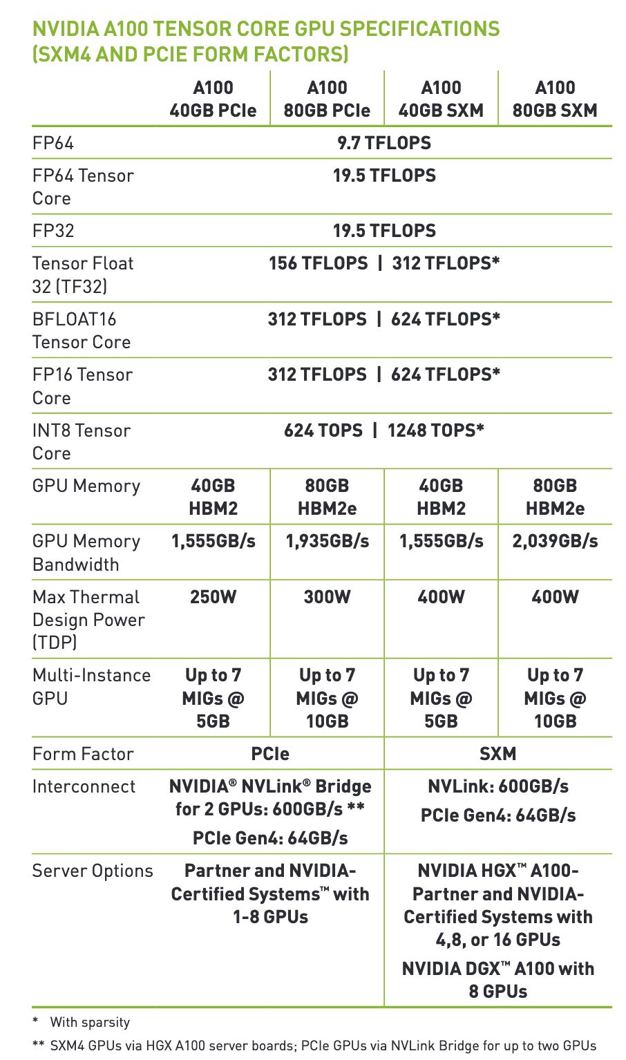
Figure 3: Specification sheet of NVIDIA A100 Tensor Core GPU. Source. The asterisk indicates the performance assuming sparsity (which is only relevant for inference).
If you cannot find the used hardware or the specifications of the mentioned hardware, we suggest referring to our sheet with estimates on the average computing capability in a given year. You can also find a chart with peak performance per year in the box below.
Imputing GPU performance when the hardware model is not known
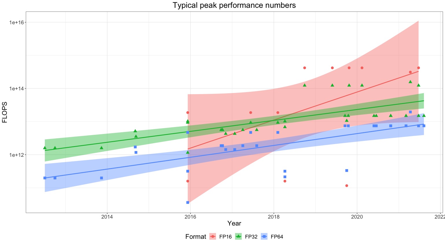
In more cases than one might expect, authors fail to report the model of GPU used in training. Unless there is no context from which we might be able to infer what hardware the authors may be using (e.g. Google tends to use TPUs), we impute missing hardware performance numbers with the averages of the peak performance numbers of GPUs used in papers published that year that meet our inclusion criteria.
Figure 4: Typical peak performance of commonly used hardware over time.
In particular, we recommend imputing missing hardware values with those in the following table, which is based on an analysis of hardware use from 35 publications in our dataset.
|
Year |
Average FP64 Performance (FLOP/s) |
Average FP32 Performance (FLOP/s) |
Average FP16 Performance (FLOP/s) |
|
2012 |
1.98E+11 |
1.58E+12 |
na |
|
2013 |
1.98E+11 |
1.58E+12 |
na |
|
2014 |
9.54E+11 |
3.35E+12 |
na |
|
2015 |
5.08E+11 |
4.96E+12 |
9.43E+12 |
|
2016 |
2.81E+12 |
6.83E+12 |
na |
|
2017 |
2.26E+12 |
5.82E+12 |
1.87E+13 |
|
2018 |
2.91E+12 |
9.37E+12 |
1.10E+14 |
|
2019 |
3.89E+12 |
6.79E+13 |
4.20E+14 |
|
2020 |
7.45E+12 |
5.81E+13 |
4.20E+14 |
|
2021 |
1.05E+13 |
6.47E+13 |
3.66E+14 |
You can find the raw data in our sheet (subsheet “PAPERS AND HARDWARE MODELS”).
Step 3: Perform the estimate
Using the extracted information from the paper and the specifications of the hardware, we can now calculate an estimate of the training compute.
\[ \text{training time} \times \text{# of cores} \times \text{peak FLOP/s} \times \text{utilization rate} \]
As the datasheet lists peak performance, we need to correct this by assuming a non-perfect utilization rate (< 100%). We suggest using a utilization rate of 0.3 for large language models, and a utilization rate of 0.4 for other networks.
About GPU utilization rates
The performance estimates on datasheets are usually theoretical peak performances — assuming full utilization and an optimal distributed workload. This is unrealistic for various reasons:
- For data intensive applications the limiting factor is the memory bandwidth and not the processing speed. Consequently, the processing speed is bottlenecked by the available bandwidth.
- When multiple GPUs are used the data needs to propagate through the network and pass through different hierarchies of memory (which come with higher latency, such as network connections).
- Memory access speed has not been improving at the same rate as processing performance. This is known as the processor-memory speed gap. Consequently, we can assume a higher utilization for smaller models (especially if they fit within the memory of a single processing unit). Whereas for bigger models where memory needs to be propagate through the network, we should assume a smaller utilization.
- Not every workload can be optimally parallelized and fully utilize the different cores of the GPU. For an optimal distribution a specific batch size, layer size, etc. is required.
Consequently, especially in multi-GPU settings, utilization rates will be much lower than 1, e.g. around 0.3. But even in simple single-GPU settings, it is very unlikely to reach utilizations over 0.75.
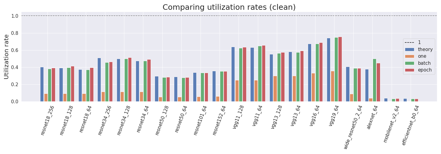
Data points for real-world utilization estimates are:
- In our experiments on different convolutional neural networks with single GPUs we observe utilization rates between 30% and 75%.
- OpenAI assumed a utilization of 33% in their piece “AI and Compute”. They assume a setup with multiple GPUs.
- A team of researchers from NVIDIA, Stanford and Microsoft achieves utilization rates between 43% and 52% for training large language models on distributed systems. This paper actively tries to maximize utilization rates. Thus, prior to 2021 rates larger than 0.5 might be hard to achieve for multi-GPU settings in LLMs. That said, there is evidence that utilization rates at top labs are rapidly improving; GSPMD reportedly yields rates as high as 62% at scale, and was recently used by Google to train LaMDA at a utilization rate of 56.5%.
- Stella Rose Biderman from EleutherAI suggests a utilization rate of around 0.4 can be achievable when training large language models on A100 GPUs.
- In the appendices of the draft report on transformative AI timelines, a 10% utilization is assumed when one “doesn’t optimize hard”, and 25%, as a reasonable ballpark, for large-scale projects where one actually tries to optimize. These are reported as subjective estimates.
- In figure 5 of (Patterson et al, 2021) the authors report GPU usage rates between 25% for GPT-3 and 39% for GShard.
To measure utilization we usually resort to a profiler. The profiler hooks onto the architecture and tries to estimate all FLOP of the network to yield a theoretical estimate. In practice however, low-level optimization routines change the training procedure in ways that differ from the theoretical setting. Thus, the true FLOP value can differ from the estimated one.
Furthermore, we found that profilers can yield very inaccurate estimates. They tend to over- or undercount and some operations are just not implemented and thus ignored. We would advise to be cautious with profiler estimates. Further comments can be found in this post.
For further discussion around metrics and utilization look at Lennart’s “Compute Research Questions and Metrics - Transformative AI and Compute [4/4]”.
Example: Image GPT
As an example we will show how to estimate the training computing of Image GPT.
In the blogpost, we find the following:
“[..]iGPT-L was trained for roughly 2500 V100-days […]“
Unfortunately, we cannot find any information about the number representation in the blogpost or paper. However, given the size, date of publication and author of this model (corporation), we assume FP16 performance.
As a next step, we need to learn about the specifications of the NVIDIA V100. We can find the datasheet easily by googling for it: NVIDIA V100 Specifications.
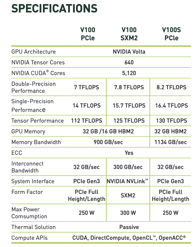
Figure 5: Specification sheet of NVIDIA V100 GPU (Source).
In the datasheet, we find three different versions of the GPU. The NVIDIA NVLink systems interface is usually used in datacenters, and I’d recommend defaulting to this option — assuming the model was authored by a company. However, the selection of which version is not that crucial, as the performance differences are rather minimal (compared to our estimates).
We find 125 TFLOPS (TFLOP/s) for the tensor core (FP16) performance. However, making full use of the tensor performance requires next to FP16 and various properties of the network architecture. See here for more on this. We should take this into consideration for the utilization.
By default, we would assume a utilization of 30% to 40%. However, given the special requirements for achieving full tensor core performance, we pick 30%.
\[ 30\% \times 125e12 \frac{FLOP}{s} \times 2500 days \times 86400 \frac{s}{day} = 8.1e21 \]
For more examples on estimating the compute used from the GPU time, see the Appendix of the blogpost AI and Compute.
Conclusion
In this article we have explained two methods for estimating the training compute in FLOP of neural network models - one based on counting the number of operations in a forward pass and another one based on GPU time.
Generally we recommend defaulting to the first method when possible - it is more exact, as GPU utilization is hard to estimate. Ideally, one would perform the estimate both ways and compare, as a sanity check6.
Over the course of this article we have produced some novel insights:
- a precise estimation of the ratio of operations between the forward and backward pass in a neural network,
- an analysis of how recurrency affects the estimation of compute,
- a table with parameter counts and forward pass FLOP for some common NN layers,
- a method of how we can estimate the training compute FLOP from the commonly shared metric GPU-days, and
- shared a best guess on the average computing capability in a given year for a single GPU.
We hope this article will help readers starting their journey into scaling laws, and help provide a reference to standardize estimations of training compute.
Acknowledgements
Thank you to Sylvain Viguier, Sasha Luccioni, Matthew Carrigan, Danny Hernandez, Girish Sastry and Stella Rose Biderman for their help answering our questions on estimating compute and GPU utilization rate.
Jean-Stanislas Denain helped us amass data about GPUs.
Thank you to Gwern Branwen and Jojo Lee for comments on the report.
Thank you to Angelina Li for spotting a minor error in the report.
Bibliography
- Alammar, Jay. 2018. “The Illustrated Transformer.” June 27, 2018.https://jalammar.github.io/illustrated-transformer/.
- Amodei, Dario, and Danny Hernandez. 2018. “AI and Compute.” OpenAI. May 15, 2018.https://openai.com/blog/ai-and-compute/.
- Chen, Mark, Alec Radford, Rewon Child, Jeff Wu, Heewoo Jun, David Luan, and Ilya Sutskever. n.d. “Generative Pretraining from Pixels,” 13.
- Cotra, Ajeya. 2020. “Draft Report on AI Timelines.” September 19, 2020.https://www.alignmentforum.org/posts/KrJfoZzpSDpnrv9va/draft-report-on-ai-timelines.
- Dumoulin, Vincent, and Francesco Visin. 2018. “A Guide to Convolution Arithmetic for Deep Learning.” ArXiv:1603.07285 [Cs, Stat], January.http://arxiv.org/abs/1603.07285.
- Narayanan, Deepak, Mohammad Shoeybi, Jared Casper, Patrick LeGresley, Mostofa Patwary, Vijay Anand Korthikanti, Dmitri Vainbrand, et al. 2021. “Efficient Large-Scale Language Model Training on GPU Clusters Using Megatron-LM.” ArXiv:2104.04473 [Cs], August.http://arxiv.org/abs/2104.04473.
- NVIDIA. 2020. “NVIDIA V100 Datasheet.” January 2020.https://images.nvidia.com/content/technologies/volta/pdf/volta-v100-datasheet-update-us-1165301-r5.pdf.
- ———. n.d. “NVIDIA A100 | Tensor Core GPU.”
- NVIDIA Documentation. n.d. “Taining With Mixed Precision - 4. Optimizing For Tensor Cores.” Concept. Training. Accessed January 19, 2022.http://docs.nvidia.com/deeplearning/frameworks/mixed-precision-training/index.html.
- Olah, Christopher. 2015. “Understanding LSTM Networks – Colah’s Blog.” August 27, 2015.https://colah.github.io/posts/2015-08-Understanding-LSTMs/.
- Patterson, David, Joseph Gonzalez, Quoc Le, Chen Liang, Lluis-Miquel Munguia, Daniel Rothchild, David So, Maud Texier, and Jeff Dean. n.d. “Carbon Emissions and Large Neural Network Training,” 22.
- Phi, Michael. 2020. “Illustrated Guide to LSTM’s and GRU’s: A Step by Step Explanation.” Medium. June 28, 2020.https://towardsdatascience.com/illustrated-guide-to-lstms-and-gru-s-a-step-by-step-explanation-44e9eb85bf21.
- Salvator, Dave. 2020. “What Is Sparsity in AI Inference and Machine Learning? | NVIDIA Blog.” The Official NVIDIA Blog. May 14, 2020.https://blogs.nvidia.com/blog/2020/05/14/sparsity-ai-inference/.
- Srivastava, Nitish, Geoffrey Hinton, Alex Krizhevsky, Ilya Sutskever, and Ruslan Salakhutdinov. n.d. “Dropout: A Simple Way to Prevent Neural Networks from Overfitting,” 30.
- TensorFlow Documentation. n.d. “Mixed Precision | TensorFlow Core.” TensorFlow. Accessed January 19, 2022.https://www.tensorflow.org/guide/mixed_precision.
Appendices
Appendix A: Profiler
In addition to the two discussed methods, one could use a profiler. A profiler is an analysis tool to measure metrics of interest. While the measurement of the number of FLOP executed is theoretically and technically possible, none of the profilers we tried (NVIDIA Nsight, PyTorch: main package and autograd) could fulfill our requirements for the training7 — many of them focus on the profiling of inference8.
Consequently, our two methods below are the method of choice, as (i) none of the existing profilers fulfills the required criteria and (ii) we require methods to estimate the compute of already published models based on the available data.
Profilers that only measure the forward pass, e.g. PyTorch’s fvcore, ptflops or pthflops, work and do their job. Our problems only arose when we tried to measure anything but the forward pass.
Appendix B: Comparing the estimates of different methods
To check whether both methods provide estimates that are consistent with one another, we compute both estimates for a few models for which this is feasible. The results (See figure below) confirm that the estimates are generally very similar (they differ by no more than a factor of 1.7).
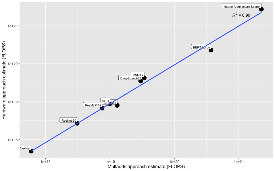
Details of these estimates may be found here.
Appendix C: Pre-training and architecture search
It is common to pre-train a large model on a large dataset and then fine-tune it on a smaller dataset. Similarly, it is common for researchers to manually train and tweak multiple versions of a system before they find the final architecture they use for training.
We recommend counting the pre-training compute as part of the total training compute.
However we do not recommend counting the tweak runs.
While these are important, for reproducibility purposes it is the pre-training and fine-tuning of the final architecture that matters most. And pragmatically speaking information on the compute used to train previous versions while finding the right architecture is seldom reported.
Appendix D: Recurrent models
The formula is more complex for recurrent models, depending on the type of recurrency.
|
Adjusting for recurrent units |
|
|
|
This is the easiest case. Since every part is repeated for each input token, we just need to adjust n_passes by a factor equal to the average amount of tokens in the set of training sequences. n_passes = n_epochs * n_batches * batch_size * avg_tokens_per_sequence training_compute = ops_per_forward_pass * 3.5 * n_epochs * n_examples |
|
|
In these cases we will need to distinguish between the recurrent and non recurrent parts of the network. training_compute = ops_per_forward_pass_recurrent * 3.5 * n_epochs * n_batches * batch_size * avg_tokens_per_sequence + ops_per_forward_pass_non_recurrent * 3.5 * n_epochs * n_examples = (ops_per_forward_pass_recurrent * avg_tokens_per_sequence + ops_per_forward_pass_non_recurrent)* 3.5 * n_epochs * n_examples We will often have that either the recurrent or non recurrent part of the network will dominate the amount of operations. In that case the formula can be suitably approximated. For example, if the non recurrent part is comparatively small, then we can approximate the compute as: training_compute ~= ops_per_forward_pass_recurrent * avg_tokens_per_sequence * 3.5 * n_epochs * n_examples |
|
|
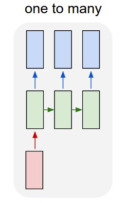
An encoder-decoder architecture can be treated as the combination of a one-to-many and many-to-one architecture. training_compute = (ops_per_forward_pass_encoder * avg_tokens_per_input + ops_per_forward_pass_decoder*avg_tokens_per_output)* 3.5 * n_epochs * n_examples |
Appendix E: Dropout
In method 1, we determined the training compute by counting the FLOP per parameter for the forward and backward passes, in order to determine the fp_to_bp_ratio. However in practice, this value is likely to vary due to regularization techniques. In this section we specifically consider the effect of dropout. This involves setting individual neurons to having a value of 0 (“dropping out”) with probability p, effectively yielding a thinned network with fewer parameters.
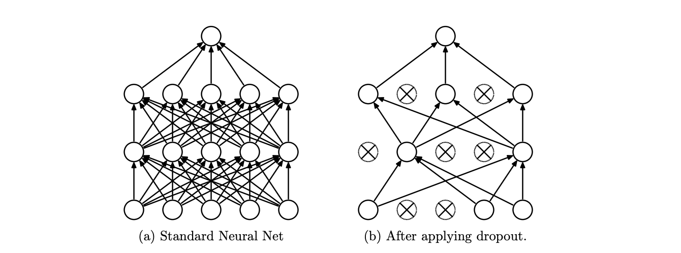
[Image source: Srivastava et al] (a) shows a standard neural network without dropout, (b) shows a thinned network, where crossed units have been “dropped out”.
Clearly this can cause the number of FLOP in a forward to decrease quite significantly, depending on the value of p, but how much exactly? In a standard neural network, the forward pass is an affine transformation and compute is dominated by the dot product if the number of neurons per layer is sufficiently large:
\[ z_i^{(l+1)} = w_i^{(l+1)} \cdot y^{(l)} + b_i^{l+1}, \]
\[ y_i^{(l+1)} = f\left(z_i^{(l+1)}\right), \]
where the symbols have their usual meanings (see for instance Srivastava et al). With dropout, the neuron value is instead a random sample drawn from a Bernoulli distribution:
\[ r_j^{(l)} \sim \text{Bernoulli}(p), \]
\[ \hat{y}^{(l)} = r^{(l)} \ast y^{(l)}, \]
\[ z_i^{(l+1)} = w_i^{(l+1)} \cdot \hat{y}^{(l)} + b_i^{(l+1)}, \]
\[ y_i^{(l+1)} = f\left(z_i^{(l+1)}\right), \]
where \( \ast \) denotes the Hadamard element-wise product. If we assume that the number of neurons is small relative to the number of parameters, then we ignore the contributions from the first two steps (random sampling and the Hadamard product), to yield roughly 2 FLOP per parameter.
What happens in the backward pass? The architecture still stays as a thinned network, and the previous consideration still holds - there are 5 FLOP per parameter in backpropagation (with the same assumptions as previously). Thus with dropout we should expect roughly the same value of 2.5 for the fp_to_bp_ratio, although perhaps adjusted slightly upward compared to the standard neural network.
Note that in addition to the fp_to_bp_ratio staying the same after dropout, ops_per_forward_pass doesn’t change by very much either. This is because dropout is typically implemented as in the equations above - by multiplying a neuron by 0 if it is to be dropped out (see for instance the TensorFlow implementation of dropout). Thus, dropout doesn’t reduce the number of operations (as one might expect if the neurons were truly removed from the network), but in fact increases it slightly, but probably not significantly. This consideration suggests that we should expect the compute implications of dropout to be quite minimal.
The inference compute is also largely unchanged - at most it is slightly increased. Generally this is implemented by multiplying the weights corresponding to the connections of a neuron by the probability p at which the neuron was dropped out. This corresponds to the same standard neural network but with a number of additional initial calculations at test time, less than or equal to the number of parameters (depending on how many neurons are dropped out).
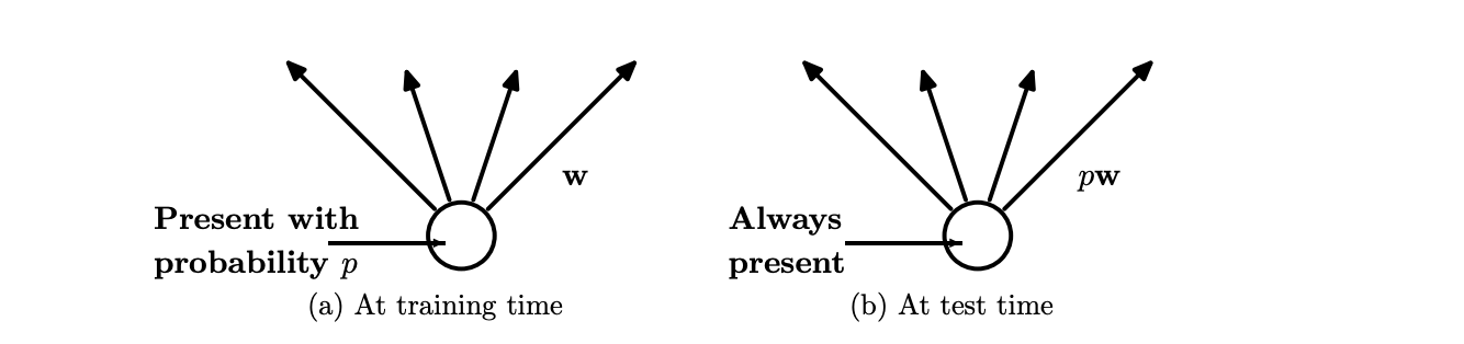
[Image source: Srivastava et al] (a) Shows dropout being implemented during training, where a neuron is dropped out with probability p. This is implemented by multiplying the neuron value by 0 if it is dropped out, and 1 otherwise. (b) Shows the same neuron at test time, where the weights of its outgoing connections are multiplied by p.
In short, it seems that other methods of regularization like using an L1 norm are likely to have a larger impact on the training compute.
-
On their website, NVIDIA states “The peak single-precision floating-point performance of a CUDA device is defined as the number of CUDA Cores times the graphics clock frequency multiplied by two. The factor of two stems from the ability to execute two operations at once using fused multiply-add (FFMA) instructions”. We interpret this statement to mean that NVIDIA used the FMA=2FLOP assumption. ↩
-
In appendix D we discuss how the formula changes when considering recurrent models. ↩
-
In appendix E we discuss the effect of dropout in the training compute. We find that in a popular implementation of dropout it does not affect the amount of operations in the forward nor backward pass. ↩
-
References: A guide to convolution arithmetic for deep learning, Illustrated Guide to LSTMs and GRUs, Understanding LSTMs, The Illustrated Transformer ↩
-
You might want to compare this to “travel-days” as a measure. Eventually, you would be interested in the distance — the quantity — so you can adjust to your means of transportations: walking, a horse, a car, etc.. Especially with computing hardware we have seen tremendous improvements in computational power over the years, so it’s relevant. ↩
-
In appendix B we show a comparison of the estimates resulting from both methods. We conclude that they are reasonably similar, and tend to be within a factor of 2 of each other. ↩
-
Marius goes into more details in the post “How to measure FLOP for Neural Networks empirically?”. It is easier to profile the forward pass but as soon as you add the backward pass, most profilers give wrong estimates. ↩
-
There is a strong interest in the use of profilers to optimize inference, as inference makes up the majority of total compute and therefore the costs (70% to 90% (Patterson et al. 2021)). ↩
About the authors


Related posts