Key takeaways

In current machine learning systems, the performance of a system is closely related to how much compute is spent during the training process. However, it is also possible to augment the capabilities of a trained model at the cost of increasing compute usage during inference or reduce compute usage during inference at the cost of lower performance. For example, models can be pruned to reduce their inference cost, or instructed to reason via chains of thought, which increases their inference cost.

Based on evidence from five concrete techniques (model scaling, Monte Carlo Tree Search, pruning, resampling, and chain of thought), we expect that, relative to most current models (eg: GPT-4) it is possible to:

1. Increase the amount of compute per inference by 1-2 orders of magnitude (OOM), in exchange for saving ~1 OOM in training compute while maintaining performance. We expect this to be the case in most language tasks that don’t require specific factual knowledge or very concrete skills (eg: knowing how to rhyme words).
2. Increase the amount of compute per inference by 2-3 OOM, in exchange for saving ~2 OOM in training compute while maintaining performance. We expect this to be possible for tasks which have a component of sequential reasoning or can be decomposed into easier subtasks.
3. Increase the amount of compute per inference by 5-6 OOM in exchange for saving 3-4 OOM in training compute. We expect this to happen only for tasks in which solutions can be verified cheaply, and in which many attempts can be made in parallel at low cost. We have only observed this in the case of solving coding problems and proving statements in formal mathematics.
4. In the other direction, it is also possible to reduce compute per inference by at least ~1 OOM while maintaining performance, in exchange for increasing training compute by 1-2 OOM. We expect this to be the case in most tasks.¹

A key implication from this work is highlighting a tradeoff between model capabilities and scale of deployment. Since inference is the dominant cost for models deployed at scale,² AI companies will apply some of these compute-saving techniques to minimize the inference costs of the models they offer to the public.³

Meanwhile, these companies might be able to leverage additional inference compute to achieve better capabilities at a smaller scale, either for internal use or for a small number of external customers. Policy proposals which seek to control the advancement or proliferation of dangerous AI capabilities should take this possibility into account.

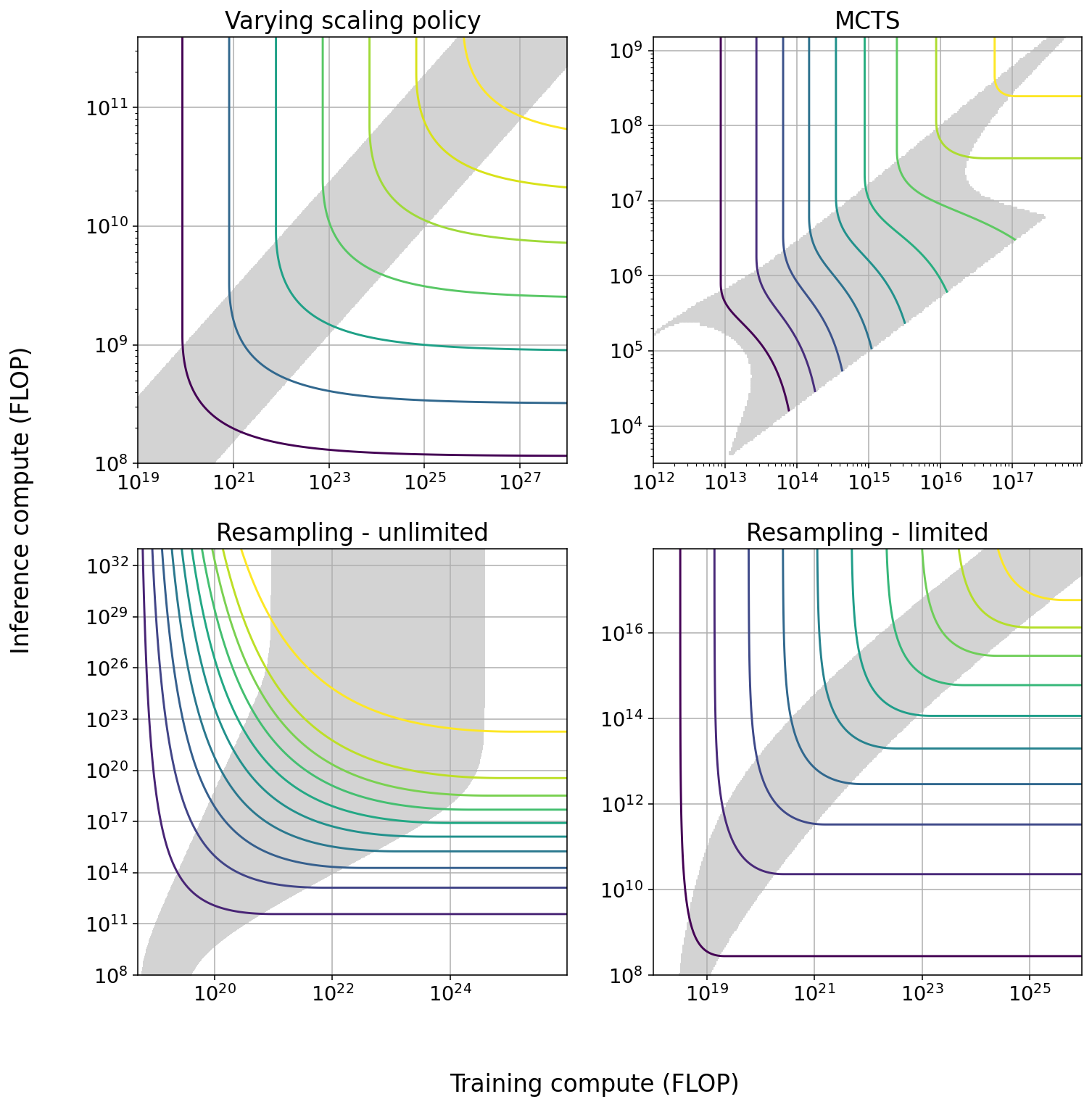
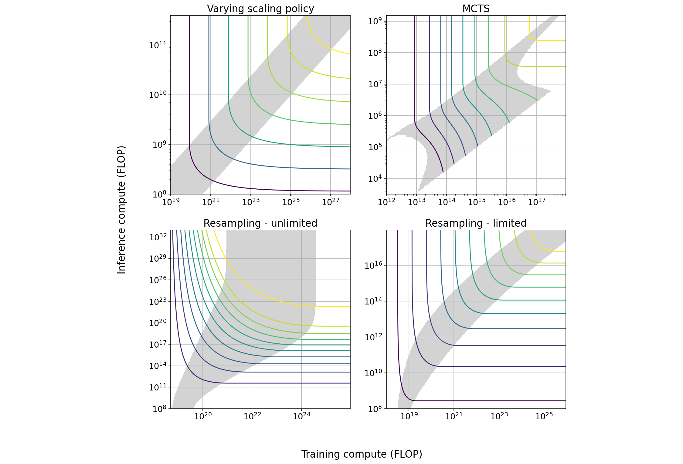
Summary Figure: Tradeoff diagrams of the four techniques we studied in greatest depth. The solid curves indicate constant performance. The shaded region is the span of efficient exchange: the region in which it is possible to trade off the two types of compute at a marginal exchange rate better than 6 to 1. In some cases the size of the span increases with scale, in others it decreases with scale.

Technique	Max span of tradeoff in training	Max span of tradeoff in inference	Effect of increasing scale	How current models are used
Varying scaling policy	1.2 OOM	0.7 OOM	None	Minimal training compute
MCTS	1.6 OOM	1.6 OOM	Span suddenly approaches 0 as model approaches perfect performance	Mixed
Pruning	~1 OOM	~1 OOM	Slightly increasing span, increasing returns to training4	Minimal training compute
Repeated sampling - cheap verification5	3 OOM	6 OOM	Increasing span6	Minimal inference compute
Repeated sampling - expensive verification	1 OOM	1.45 OOM	None	Minimal inference compute
Chain of thought	NA7	NA	Unknown	Minimal inference compute

Summary Table: For each of the five techniques we studied, we display: the maximum size of the tradeoff in both training and inference compute; how the tradeoff behaves as models are scaled; and in which region of the tradeoff current models usually stand. ‘Minimal training compute’ indicates that current models are trained using as little training compute as possible given their performance.

Overview

Introduction

The relationship between training compute and capabilities in machine learning systems is well known, and has been extensively studied through the lens of scaling laws.⁸ This relationship is responsible for the current concentration of advanced AI capabilities in companies with access to vast quantities of compute. It is also used for forecasting AI capabilities, and forms the technical foundation for some proposed policies designed to control the advancement and proliferation of frontier AI capabilities.⁹

Less attention has been paid to the effect of inference compute on capabilities. While this effect is limited, we argue that it is significant enough to warrant consideration. There are multiple techniques that enable spending more compute during inference in exchange for improved capabilities. This possibility induces a tradeoff between spending more resources on training or spending more resources on inference.

The relationship between training and inference compute is complex: we must distinguish between the cost of running a single inference, which is a technical characteristic of the model, and the aggregate cost of all the inferences over the lifetime of a model, which additionally depends on the number of inferences run.

The cost of running a single inference is much smaller than the cost of the training process. A good rule of thumb is that the cost of an inference is close to the square root of the cost of training (see Figure A), albeit with significant variability.¹⁰ Meanwhile, the aggregated cost of inference over the lifetime of a model often greatly exceeds the cost of training, because the same model is used to perform a large number of inferences.¹¹

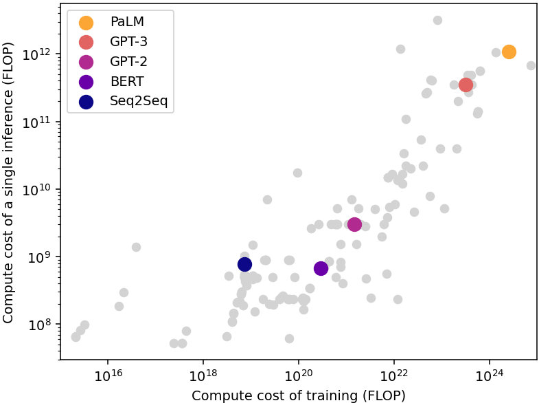
Figure A: Compute required for training and running a single inference of multiple language models published since 2012. The single-inference compute is usually close to the square root of the training compute. Data from Epoch AI (2022).

The tradeoff

Individual techniques

We analyzed several techniques that make it possible to augment capabilities using more inference compute, or save inference compute while maintaining the same performance. The quantities of compute which can be traded off vary by technique and domain.

For example, using overtraining, it’s possible to achieve the same performance as Chinchilla, spending 2 OOMs of extra training compute in order to save 1 OOM of inference compute. Meanwhile, using resampling it’s possible to achieve the same performance as AlphaCode spending 1.5 OOM of additional inference compute in order to save 1 OOM of training compute. Both of these possibilities are illustrated in Figure B, which presents the tradeoff induced by these two concrete techniques.

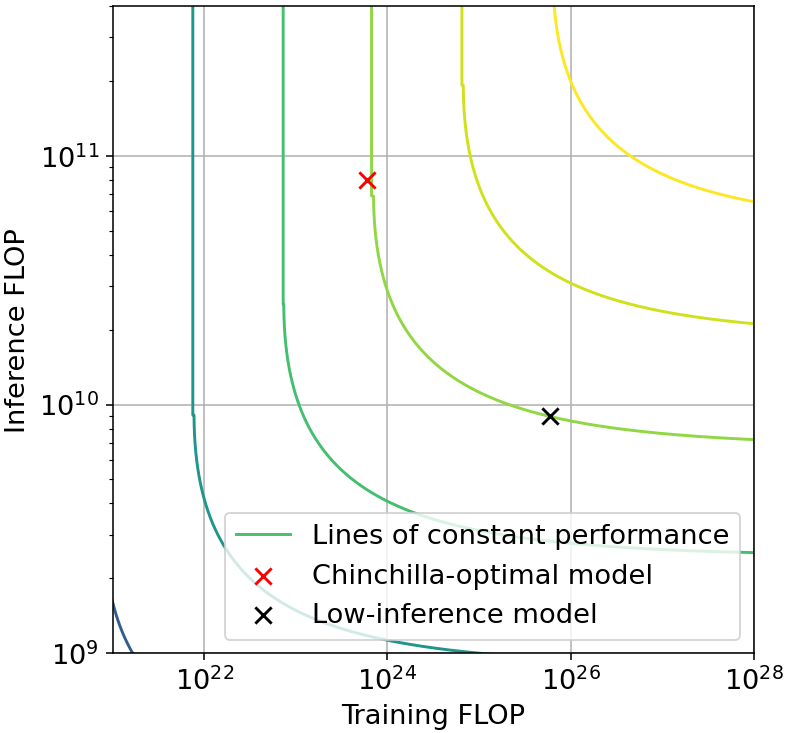
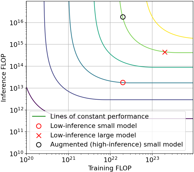
Figure B: Illustrative tradeoff examples. Left: tradeoff from overtraining in language modeling. The low-inference model (black) saves one order-of-magnitude (OOM) in inference by spending 2 additional OOMs in training, relative to a Chinchilla-optimal model. Right: tradeoff from resampling in n@k code generation. The high-inference model (red circle) saves 1 OOM in training compute by spending an additional 1.5 OOM in inference compute, relative to a non-augmented model (red x). Since augmentation can be done post-training, this means that a small model (red circle) can simulate the capability of a 1 OOM larger model, after being augmented with 3 OOM of additional inference compute.

Since there is significant variation between techniques and domains, we can’t give precise numbers for how much compute can be traded off in a general case. However, as a rule of thumb we expect that each technique makes it possible to save around 1 OOM of compute in either training or inference, in exchange for increasing the other factor by somewhat more than 1 OOM.

In addition, there is a class of tasks in which inference compute can be leveraged quite efficiently. In tasks where the solution generated by the AI can be cheaply verified and where failures are not costly (for example, writing a program that passes some automatic tests, or generating a formal proof of a mathematical statement) it is possible to generate a large number of solutions until a valid one is found.

For these tasks, it is possible to usefully spend an additional 6 orders of magnitude of compute during inference, and reduce training compute by 3 orders of magnitude. While we don’t expect many economically relevant tasks will have these characteristics, there might be a small number of important examples.¹²

Combining techniques

These techniques can be combined. We verified that at least in some cases, the effect of combining two techniques is as large as the combination of the individual effects. That is, if each technique allows 1 OOM of savings, using both techniques in combination allows 2 OOM of savings.

However, we believe this is a special case, and in general combining two techniques will produce less benefits than the sum of each individual technique. This is because each of these techniques can interfere with each other if they use the same mechanism of action.¹³ Therefore, we expect that only techniques which employ very different mechanisms of action will combine effectively.

After taking this into account, we believe using combinations of techniques can allow up to around 2-3 OOM of savings, because combining more than two techniques will usually be ineffective.¹⁴ Some of these techniques (in particular Chain of Thought and MCTS) seem to mostly produce benefits for tasks which have a compositional structure, like sequential reasoning. Other tasks might not see such large savings.

Implications

The position of current models in these tradeoffs is crucial to evaluate their consequences. If current models are near the maximum inference compute for all techniques, it will be possible to save a lot of inference compute but no training compute at all, and vice versa.

The past generation of LLMs (GPT-3, PaLM, Chinchilla) would be placed close to a middle point in the combined tradeoff. This is because in each technique they are often in one of the extremes of the tradeoff, but they are in different extremes for different techniques. They use no pruning and no overtraining, so they are in the extreme of high inference compute for those techniques, but they also use no chain of thought or search, so they are in the extreme of low inference compute for those techniques.

While we know less about the latest-generation models (GPT-4, PaLM 2), and nothing about future models, we think they are likely to stand closer to the low-inference end of the combined tradeoff, for the following reason:

The optimal balance between spending compute on training or inference depends on the number of inferences that the model is expected to perform. In applications which are expected to require a large number of inferences (eg: deploying a system commercially), there is an economic incentive to minimize inference costs. In the opposite case, for applications which are expected to only require a small number of inferences (eg: evaluating the capabilities of a model), there is no such incentive since training is the dominant cost.¹⁵

As a consequence, it seems likely that models deployed at scale will be closer to the low end of inference compute. Meanwhile, there will be substantially more capable versions of those models that use more inference compute and therefore won’t be available at scale.

Conclusions

Spending additional compute during inference can have significant effects on performance. This is particularly true for models deployed at scale by AI companies or open source collectives, which have an incentive to produce models that are optimized for running cheaply during inference.

In some cases, it might be possible to achieve the same performance as a model trained using 2 OOM more compute, by spending additional compute during inference. This is approximately the difference between successive generations of GPT models (eg: GPT-3 and GPT-4), without taking into account algorithmic progress. Therefore it should be possible to simulate the capabilities of a model larger than any in existence, using current frontier models like GPT-4, at least for some tasks. Even larger improvements might be possible for tasks where automatic verification is possible.

This has several consequences for AI governance. While these amplified models will not be available at scale, some other actors might be able to leverage them effectively. For example:

1. Model evaluations and safety research can use these techniques to anticipate the capabilities that will become available at scale in the future.
2. AI progress might be faster than expected in some applications, at a limited scale due to higher inference costs. For example, AI companies might be able to use augmented models to speed up their own AI research.

Full report

Background

For a given machine learning model and training setup, there is usually a fixed ratio between compute spent in training and compute spent in a single inference, determined by the architecture, optimization method, and quantity of training data, among other things.

However, for certain kinds of models and tasks this compute expenditure can be modified, such that we can independently vary the amount of compute spent in training and inference. In addition, sometimes simply running the model more than once for each inference can help. In this way, we can trade off less compute spent on training for more compute spent on inference, or vice versa, without affecting performance.

This has implications for predicting compute requirements for AI automation. For example, it might be possible to achieve human-level AI using much less compute during training, in exchange for more expensive inferences.

Contributions

A preliminary report identified several techniques that enable this tradeoff, did some preliminary analysis of each technique, and considered using a CES function for modeling the tradeoff. The report concluded that a CES function might not capture the tradeoff dynamics well enough.

In this report, we selected a subset of those techniques for which enough data is available to perform scaling analyses with respect to both training and inference compute. We then fit different functional forms to the data, informed by the particular scaling behavior of each technique and analyze the tradeoff based on the fitted models.

The four techniques we selected are: model and data scaling, Monte Carlo tree search (MCTS), pruning, and multiple sampling. Each of these techniques has an associated control variable which determines whether the model is more compute-heavy or inference-heavy. Some of these variables are bounded, for example, one cannot generate less than one sample per inference. These bounds translate to limitations in the tradeoff.

	Techniques
Technique name	Varying the scaling policy	Pruning	MCTS	Sampling + selection
Control variable	Data/parameter ratio	Density of pruned model	Number of MCTS nodes	Number of samples
Mechanism	Number of parameters	Number of parameters	Number of forward passes	Number of forward passes
Domain of study	Language	Vision	Games	Language

Table 1: Techniques we studied and their characteristics. Mechanism refers to what mediates the influence of each technique on inference compute. Domain of study is the particular domain of the models we used to study each technique (but note that all of them can be applied to several domains).

Techniques

Varying the scaling policy

Just by modifying the number of parameters of the model and the size of the training dataset, it is possible to obtain a model with a desired training and inference compute, within certain limitations. The training compute TC and inference compute IC are roughly related to the number of parameters N and the amount of data D by the following relations: TC = 6ND, IC = 2N.

Using these relations, we can derive an equation for the tradeoff from a scaling law in terms of N and D. As an example, the scaling law found in Hoffmann et al. (2022) is

\[ L = E + AN^{-a} + BD^{-b} = E + A(IC/2)^{-a} + B(TC/3IC)^{-b} \]

By substituting the values of the parameters found empirically, we can see that this allows for a reduction of about 0.7 OOM (order of magnitude) in the inference compute, in exchange for spending about 1.2 OOM more in training. This can be worth it at relatively small scales if the model is going to be used for many inferences (Figure 2).¹⁶ However, this tradeoff can’t be used to save training compute, as current models are already being trained with minimal compute.

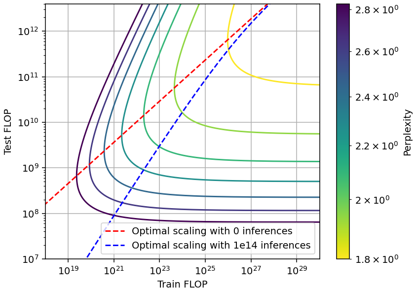
Figure 2: Shape of the tradeoff induced by the scaling laws from Hoffmann et al. (2022). The red dashed line corresponds to Chinchilla scaling, the blue dashed line corresponds to compute-optimal scaling, taking into account the cost of performing 1e14 inferences.

An interesting feature of this type of tradeoff is that at the extreme of high inference compute, the contour lines are not vertical but diagonal. This is because increasing inference compute at a constant level of training compute would require training on less data, which hurts performance. Thus, to maintain performance, training compute must increase with inference compute.

Meanwhile, we can increase training compute just by training on more data, which does not affect inference compute at all. For this reason, the contour lines stay horizontal at the extreme of high training compute.

Monte Carlo Tree Search

Some game-playing agents, particularly AlphaZero, employ Monte Carlo Tree Search (MCTS) during their forward pass (Silver et al., 2017). The number of nodes of this search can be modified between training and inference, and the total compute per forward pass is proportional to this number.¹⁷

To study the scaling of MCTS agents, we replicated and extended the results in Jones (2021). We evaluated AlphaZero agents of different sizes and different MCTS nodes trained on the turn-based board game Hex.¹⁸

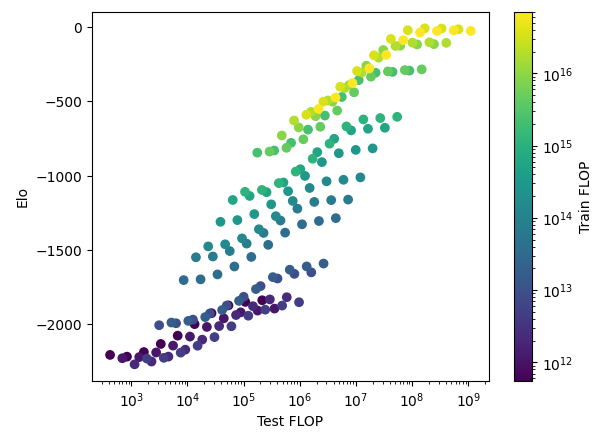
Figure 3: Scaling of AlphaZero agents in Hex is an S-curve in terms of both test FLOP and train FLOP (notice the concentration of points at both high and low ends of train FLOP).

The performance of the agents behaves as an S-curve in both training compute and in the number of MCTS nodes (Figure 3). From this relationship, we can derive a scaling law:

\[ ELO = E+ \sigma(\log(C)) + \sigma(\log(M)) \]

Where σ is any parametrization of an S-curve that can fit the data, C is the training compute, and M is the number of MCTS nodes. In our case, we used a smoothly broken power law (Caballero et al., 2022) to parametrize an S-curve.

\[ \sigma(C) = a(x_0 - x_1) + d_0 \log(1 + \exp((C - x_0)/d_0)) - d_1 \log(1 + \exp((C - x_1)/d_1) \]

The parameters of these curves depend on the scaling policy of the models, and for this reason, we fit our model only to a subset of the data, composed by models trained with a specific scaling policy. This allows us to isolate the effect of changing just the number of MCTS nodes, separate from the effect of changing the scaling policy.

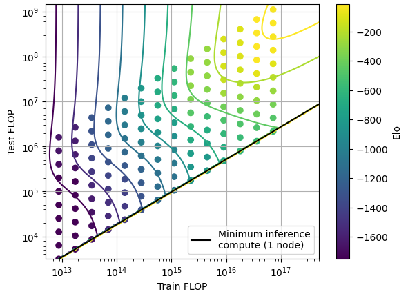
Figure 4: Model contour lines and empirical data for MCTS tradeoff in Hex. Elo is normalized so that perfect play corresponds to 0 points, and lower Elo corresponds to lower performance.

Using this scaling law we can plot the shape of the tradeoff (Figure 4). Since we can’t run models with less than 1 MCTS search node, there is a minimum inference compute for each training compute.

In this case, the slope and span of the tradeoff is constant at small scales, but changes at larger scales when the models approach perfect play. This change in shape is due to the fact that scaling model size alone is not enough to reach perfect performance. Increasing the number of MCTS nodes becomes necessary to improve performance beyond -500 Elo, and as a consequence the span of the tradeoff is reduced.

At low performance we trade off a bit more than 1.6 OOM in inference for 1 OOM in training. Meanwhile, at high performance this almost reverses: we can trade off 1.6 OOM in training for just 1.1 OOM in inference (Figure 5). Finally, as we reach perfect performance, the tradeoff disappears and there is a single point which minimizes both training and inference compute.

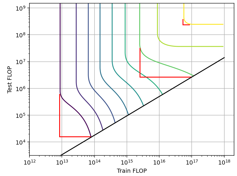
Figure 5: The span of the MCTS tradeoff changes with scale

In addition, we see that in the extreme of high training compute, the contour lines are not horizontal (at high performance at least), while in the extreme of high inference compute, the lines are vertical. This is the opposite of what we saw in the case of Chinchilla scaling, because in this case, we can freely increase inference compute without reducing training compute (by adding MCTS nodes), but not the other way around.

Pruning

Pruning refers to a set of techniques for reducing model size after training by removing irrelevant weights (Blalock et al., 2020). While this technique can’t be used to save compute in training, it can be used to save compute in inference. We only analyzed Iterative Magnitude Pruning (IMP) (Frankle et al., 2018), a concrete pruning technique for which we could find scaling analyses.

This technique works as follows: the model is trained as usual, and then a fraction of weights with smallest magnitude are set to zero. Then, the remaining weights are reset to their initialization values, and the model is trained again. This process is repeated several times. A common setup is pruning 20% of the weights in each iteration and running up to ~20 iterations (Frankle et al., 2018).

The density of the pruned model is the ratio of pruned size to unpruned size, or the percentage of weights remaining after pruning. Since inference compute is proportional to model size, decreasing the density reduces inference compute by the same factor.

However, pruning increases the cost of training, as after each pruning iteration, the model must be trained again. If a fraction x of the weights are pruned at each iteration for n iterations, then the training compute increases by a factor of (1-(1-x)^n)/x. For example, to achieve a density of 10% while pruning 20% of the weights, each round requires about 4.5x as much training compute.

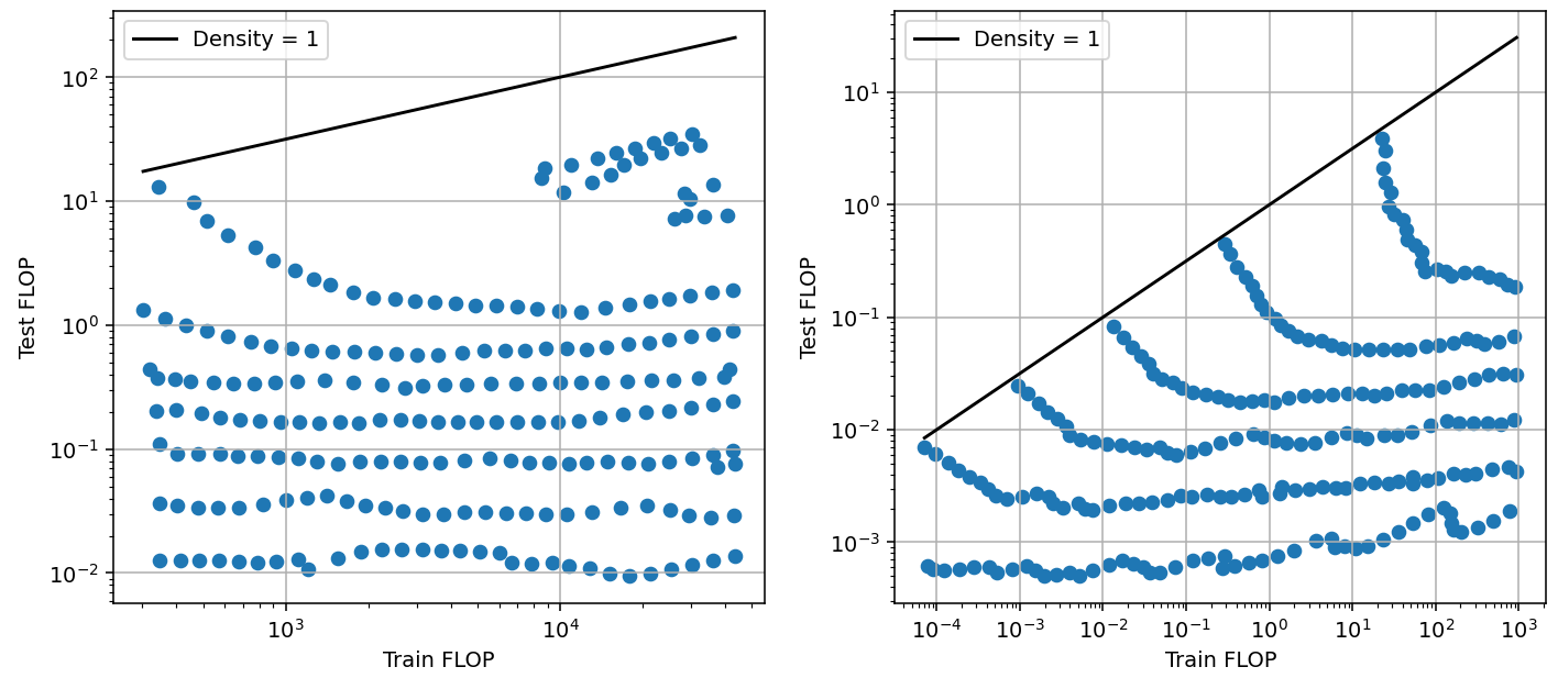
Figure 6: Tradeoff for pruning, using data from Rosenfeld et al. (2020). Left: scaling network depth (number of layers). Right: scaling network width (size of layers). We include the cost of pruning as part of the training compute.

We see that the characteristics of the tradeoff change with scale (Figure 6, right). Larger models can be pruned further, saving more inference compute in exchange for less training compute. At the largest scale tested, pruning can reduce inference compute by about 1 OOM with only a ~0.7 OOM increase in training compute, while maintaining performance. This corresponds to pruning models to a density of about 10%. This dependence on scale might reflect that the model is overfitting at the largest scales and benefits more from pruning.

Repeated sampling and filtering

In generative models, it is possible to sample the model more than once and keep only the best of the generated outputs. In the particular case of solving coding problems, this substantially increases the probability of producing a correct answer (Li et al., 2022).

We gathered data on code and math generation. In these domains, the correctness of the solution can be evaluated automatically, which makes large-scale sampling practical. There are two types of metrics for these problems:

• pass@k is the probability that, after generating k samples, any of them is correct
• n@k is the probability that, after generating k samples and selecting n of them, any of those n is correct.

n@k is used to simulate the conditions in other domains where checking the correctness of the solution is costly, and thus only a small number of candidate solutions can be evaluated. In this setting, the generated samples are filtered according to some quality criteria until only n of them are left.

When using pass@k, adding more samples always helps, since there’s always a chance that one of those is correct. However, this is not true for n@k. If the filtering does not always select the best samples, and the value of n is small enough, then increasing the number of samples eventually leads to a plateau (Figure 7).

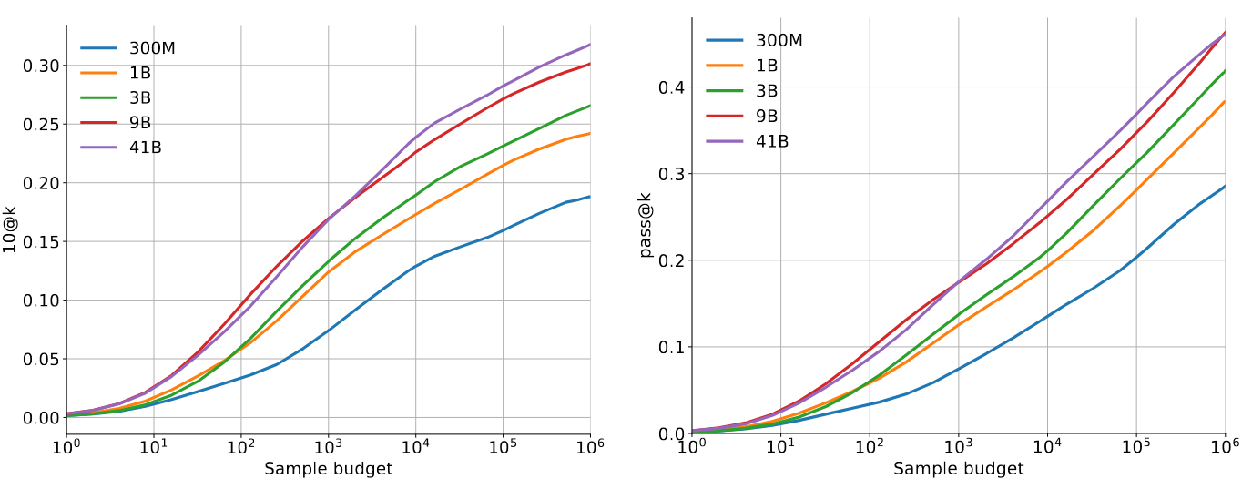
Figure 7: Comparison between 10@k and pass@k in AlphaCode, for different model sizes and values of k (sample budget). Source: Li et al. (2022).

Unlimited Trials

We can model the situation with pass@k as follows: accuracy is a power law function of some measure of “exploration.” Increasing the number of samples increases the amount of explored solutions, and larger models explore better. This last part can be represented by a simple logarithmic function, where the exploration value of a sample is \(b = a \log TC + A\), where TC is the training compute and A,a are parameters to be fitted. Then, performance is given by an S-curve with slope b, parametrized by a smoothly broken power law, slightly modified so that the curve always saturates at 100% accuracy:

\[ P(\log IN) = b(d_0 \log(1 + \exp((\log IN - x_0)/d_0) - d_1 \log(1 + \exp((\log IN - 1/b - x_0)/d_1)) \]

We tested this model on the AlphaCode results. Despite its simplistic assumptions, it fits the data reasonably well (Figure 8).

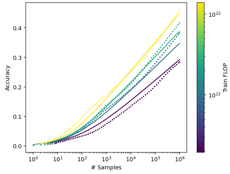
Figure 8: Scaling model for code generation using pass@k. The dots represent real data, while the solid lines are the model fit. Data from Li et al. (2022).

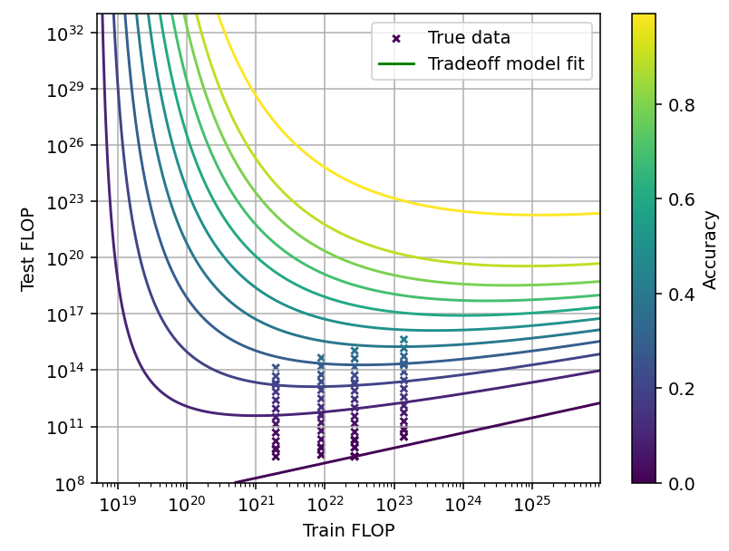
Figure 9: Tradeoff for code generation using pass@k. Data from Li et al. (2022).

Using this model, we can plot the shape of the tradeoff for pass@k. Unfortunately, the data is quite limited so we should not take this model very seriously. However, it seems the shape of the tradeoff depends on scale. At small scales we can trade off up to 2 OOM in training for about 3-4 OOM in inference. Meanwhile, at close to perfect accuracy we can trade off 4 OOM in training for just 6 OOM in inference (Figure 9). The overall shape of the tradeoff is similar to the MCTS case, with the contour lines sloping upwards in the limit of high training compute.

In addition to AlphaCode data, we also tested our model on math generation data from Minerva (Figure 10). In this case, performance for pass@k behaves very similarly to the n@k case, with accuracy plateauing at a certain number of samples. It seems plausible that we would observe the same behavior in AlphaCode, with enough samples. If this is true, then the model we sketched above would be invalid, and we’d have to use the same model we develop below for limited trials.

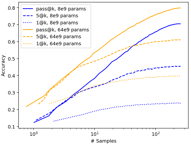
Figure 10: pass@k and n@k performance for Minerva. Data from Lewkowycz et al. (2022).

Limited trials

In the case of n@k, adding more samples eventually stops improving performance. We use a very similar model to the previous case, the only difference being that the S-curve saturates to a value smaller than 1 and given by the slope b.

\[ P(\log IN) = b (d_0 \log(1 + \exp((\log IN - x_0)/d_0) - d_1 \log(1 + \exp((\log IN - x_1)/d_1)) \]

As a consequence of this difference, we can only trade off about 1 OOM in training and 1.45 OOM in inference (Figure 11). It also seems to be independent of scale, though we have low confidence in this conclusion since the data does not cover many orders of magnitude.

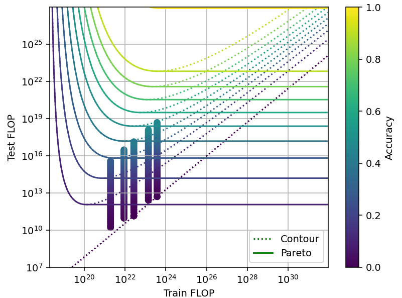
Figure 11: Tradeoff for code generation using 10@k. Data from Li et al. (2022).

Chain of thought and model cascades

The term “language model cascade” (Dohan et al., 2022) refers to the structured composition of multiple language model inferences, encompassing techniques like scratchpads, task decomposition and delegation, reflexion, etc.

While these techniques significantly improve performance in some tasks by employing more inference compute, we did not analyze them quantitatively. This is partly because we could not find much data of how these techniques scale with more inference compute. In addition, a lot of these techniques don’t admit continuous changes in intensity of usage, but only a discrete change from not using the technique to using it. Therefore, our approach of fitting tradeoff curves is not well suited to model these techniques.

The most illustrative data of this kind we found was for Tree-of-Thoughts (Yao et al., 2023).¹⁹ This technique consists of a search over chain-of-thought reasoning paths, and is reminiscent of MCTS. In fact, its behavior with scale seems similar to that of both MCTS and sampling+selection, with accuracy increasing log-linearly in the number of nodes.

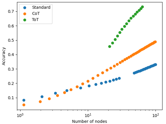
Figure 12: Tree-of-Thoughts scaling with the number of search nodes, compared to Chain-of-Thought and standard prompting (in those cases, the number of nodes is just the number of generated samples). Data from Yao et al. (2023).

Combining tradeoffs

Some of these techniques can be used in combination, which would lead to larger tradeoffs. For example, in the case of Hex we have data for both the Chinchilla-style tradeoff and the MCTS tradeoff, and we can compare the extent of those two separately and combined (Figure 13). The span of the combined tradeoff is close to the sum of the two independent spans.

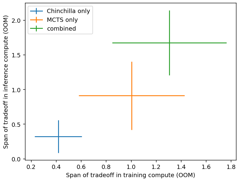
Figure 13: Combination of tradeoffs for Hex. The position and size of the crosses indicate the mean and standard deviation taken across different performance levels. Data from Jones (2021).

Presumably, not all of the techniques we studied can be combined effectively. That is, combining some of these techniques won’t lead to a larger tradeoff. We speculate that the Chinchilla and pruning techniques can’t be effectively combined, since they both employ the model size as an independent parameter. Similarly, the MCTS and resampling techniques probably can’t be combined either, since they both involve repeated queries to the model.

Modeling the tradeoff

When studying the tradeoff produced by each technique, we observed that it is generally possible to achieve a worse performance after increasing both training and inference compute. That is, the contour lines we have been plotting so far are not Pareto frontiers. We paid attention to these inefficient training configurations because they help fit our models to the data.

However, we would expect actual researchers to use the optimal training configuration that is available with their training and inference compute budgets. So for our tradeoff model, we will pay attention only to the pareto frontiers, and not the actual contour lines of the loss (Figure 14).

Figure 14: Pareto frontiers vs contour lines of the loss

From our study of the tradeoff produced by different techniques, we have identified three qualitatively different types of tradeoffs (Figure 15). The relevant differences between them are 1) whether performance saturates with respect to training or inference compute when keeping the other constant, and 2) whether the span of the tradeoff is constant or decreases with scale.

We are likely to see decreasing spans with scale when we are close to reaching perfect performance for the task at hand, as we see with Hex and MATH. Meanwhile, when we could continue scaling models for many orders of magnitude without reaching a plateau, we tend to see constant spans.

1. Saturating, constant span with scale. Example: Chinchilla scaling. We are likely to see this kind of tradeoff when the models are still far from reaching perfect performance. This type of tradeoff can be modeled with a CES function.
2. Saturating, decreasing span with scale. Example: MCTS, code generation with limited attempts. We are likely to see this kind of tradeoff when the models are close to reaching perfect performance. This might be well modeled by a logarithmic CES function.
3. Non-saturating, increasing span with scale. Example: code generation with unlimited attempts. This is a very different kind of tradeoff that arises when performance as a function of training or inference compute does not plateau when keeping the other factor constant. That is, adding more compute always helps. This can be modeled with a hyperbolic function.

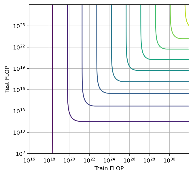
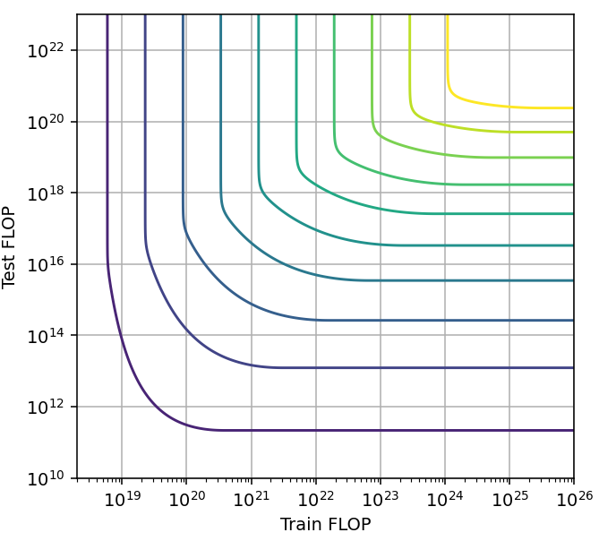
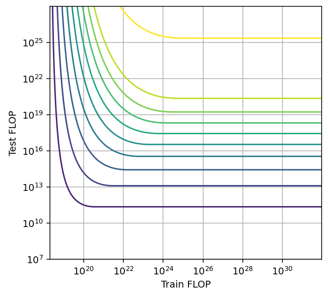
Figure 15: Pareto frontiers for tradeoff types a, b and c (left to right).

The only plausible instance of a tradeoff of type c) is code generation with unlimited retries. In this case, the returns to inference compute don’t seem to reach zero even after increasing for six orders of magnitude. However, in an easier math generation benchmark, we do see that returns to extra inference compute eventually reach zero. This suggests that code generation performance will also saturate with enough inference compute, even if we have not yet reached that point.

Pruning seems to be another technique for which the span increases with scale. However, we believe this to be an artifact of overfitting and don’t expect the pruning tradeoff to behave the same way for harder tasks or generative models.

Efficiency and optimal scaling

The efficiency of the tradeoff refers to the “exchange rate” between training and inference compute. Over the full span of the tradeoff, the efficiency is usually somewhat below 1, so that saving 1 OOM in either training or inference requires increasing the other factor by more than 1 OOM. However, the efficiency is not uniform in general over the span of the tradeoff, and the optimal point will vary depending on the relative cost of training and inference compute.

Conclusion

From our study of four different techniques, we have identified several qualitative and quantitative properties of the training/inference compute tradeoff. We expect this tradeoff to maintain a constant or decreasing span when increasing scale in most cases, and we expect this span to be around one or two orders of magnitude in both factors.

A possible exception to this is the case of resampling with unlimited trials, in which returns to additional inference compute are always significant, and in which it seems possible to achieve much larger spans (six orders of magnitude or more) which are increasing with scale. However, we only reach this conclusion by extrapolating the scaling law over twice the range in which it was fit. Moreover, results in easier math generation benchmarks don’t show these increasing spans. As a consequence, we currently have low confidence that the resampling technique with unlimited trials will be as promising as we indicate.

Some of the above techniques can be combined to yield tradeoff spans of two or three orders of magnitude. Additional techniques might be discovered that can be combined with existing ones, but as long as those new techniques induce similar tradeoffs to the known ones, we do not expect to see tradeoffs spanning more than three to four orders of magnitude.

Acknowledgements

We would like to thank Ege Erdil, David Owen, Anson Ho, Tom Davidson, Tamay Besiroglu, Jean-Stanislas Denain, Jaime Sevilla, Markus Anderljung and Lisa Soder for their comments on earlier versions of this draft.

Bibliography

Blalock, D., Ortiz, J. J. G., Frankle, J., & Guttag, J. (2020). What is the State of Neural Network Pruning? ArXiv:2003.03033 [Cs, Stat]. https://arxiv.org/abs/2003.03033

Caballero, E., Gupta, K., Rish, I., & Krueger, D. (2023, July 23). Broken Neural Scaling Laws. ArXiv.org. https://doi.org/10.48550/arXiv.2210.14891

Dey, N., Gosal, G., Chen, Z., Khachane, H., Marshall, W., Pathria, R., Tom, M., Hestness, J. (2023). Cerebras-GPT: Open Compute-Optimal Language Models Trained on the Cerebras Wafer-Scale Cluster. ArXiv:2304.03208 [Cs]. https://arxiv.org/abs/2304.03208

Dohan, D., Xu, W., Lewkowycz, A., Austin, J., Bieber, D., Lopes, R. G., Wu, Y., Michalewski, H., Saurous, R. A., Sohl-dickstein, J., Murphy, K., & Sutton, C. (2022, July 28). Language Model Cascades. ArXiv.org. https://doi.org/10.48550/arXiv.2207.10342

Epoch AI. (2022). Parameter, Compute and Data Trends in Machine Learning. /data/epochdb/table

Frankle, J., & Carbin, M. (2019). The Lottery Ticket Hypothesis: Finding Sparse, Trainable Neural Networks. ArXiv:1803.03635 [Cs]. https://arxiv.org/abs/1803.03635

Jones, A. L. (2021, April 15). Scaling Scaling Laws with Board Games. ArXiv.org. https://doi.org/10.48550/arXiv.2104.03113

Lewkowycz, A., Andreassen, A., Dohan, D., Dyer, E., Michalewski, H., Ramasesh, V., Slone, A., Anil, C., Schlag, I., Gutman-Solo, T., Wu, Y., Neyshabur, B., Gur-Ari, G., & Misra, V. (2022). Solving Quantitative Reasoning Problems with Language Models. ArXiv:2206.14858 [Cs]. https://arxiv.org/abs/2206.14858

Li, Y., Choi, D., Chung, J., Kushman, N., Schrittwieser, J., Leblond, R., Eccles, T., Keeling, J., Gimeno, F., Dal Lago, A., Hubert, T., Choy, P., de Masson d’Autume, C., Babuschkin, I., Chen, X., Huang, P.-S., Welbl, J., Gowal, S., Cherepanov, A., & Molloy, J. (2022). Competition-level code generation with AlphaCode. Science, 378(6624), 1092–1097. https://doi.org/10.1126/science.abq1158

Olausson, T. X., Inala, J. P., Wang, C., Gao, J., & Solar-Lezama, A. (2023, June 22). Demystifying GPT Self-Repair for Code Generation. ArXiv.org. https://doi.org/10.48550/arXiv.2306.09896

Owen, D. (2023). Extrapolating performance in language modeling benchmarks. https://epochai.org/files/llm-benchmark-extrapolation.pdf

Patterson, D., Gonzalez, J., Urs Hölzle, Le, Q. V., Liang, C., Lluís-Miquel Munguía, Rothchild, D., So, D. R., Texier, M., & Dean, J. (2022). The Carbon Footprint of Machine Learning Training Will Plateau, Then Shrink. ArXiv (Cornell University). https://doi.org/10.48550/arxiv.2204.05149

Rosenfeld, J. S., Frankle, J., Carbin, M., & Shavit, N. (2021, July 3). On the Predictability of Pruning Across Scales. ArXiv.org. https://doi.org/10.48550/arXiv.2006.10621

Silver, D., Hubert, T., Schrittwieser, J., Antonoglou, I., Lai, M., Guez, A., Lanctot, M., Sifre, L., Kumaran, D., Graepel, T., Lillicrap, T., Simonyan, K., & Hassabis, D. (2017). Mastering Chess and Shogi by Self-Play with a General Reinforcement Learning Algorithm. ArXiv.org. https://arxiv.org/abs/1712.01815

Yao, S., Yu, D., Zhao, J., Shafran, I., Griffiths, T. L., Cao, Y., & Narasimhan, K. (2023, May 17). Tree of Thoughts: Deliberate Problem Solving with Large Language Models. ArXiv.org. https://doi.org/10.48550/arXiv.2305.10601

Zelikman, E., Huang, Q., Poesia, G., Goodman, N. D., & Haber, N. (2023, May 28). Parsel: Algorithmic Reasoning with Language Models by Composing Decompositions. ArXiv.org. https://doi.org/10.48550/arXiv.2212.10561

Notes

1. Since the techniques we have investigated that make this possible, overtraining and pruning, are extremely general. Other techniques such as quantization also seem very general ↩

2. Patterson et al. (2022) find that the aggregate cost of inference at Google data centers in three weeks of 2019, 2020 and 2021 accounts for 60% of the total ML compute expenditure. In addition, the fact that as of july 2023 GPT-4 is only available with a rate limit in ChatGPT, even for paying customers, suggests that inference is currently a bottleneck for AI companies. ↩

3. This is already the case, with quantization being commonly used in open-source models, and speculatively also in closed-source models. ↩

4. Span in inference compute increases by roughly 0.08 OOM for each OOM increase in training compute. The efficiency of the tradeoff (the ratio of inference compute reduction to training compute increase) increases by 0.5 for each OOM increase in training compute. ↩

5. Note that we are extrapolating over many orders of magnitude and we should treat this result with skepticism. ↩

6. Span in both training and inference compute increases by 0.75 OOM for each OOM increase in training compute. ↩

7. We could not determine this quantity for chain of thought-style techniques, since they are usually binary: either they are employed or not, with no possibility of continuous variation in the intensity of usage. ↩

8. See, for example, Owen (2023) ↩

9. Some examples are the proposed moratorium on training runs beyond a certain size, and the proposal to require a license to train large models. ↩

10. For example, for GPT-3, the cost of training was 3e23 FLOP, whereas the cost of a single inference is 3e11. So the cost of training is equivalent to performing 1e12 inferences. ↩

11. Patterson et al. (2022) find that the aggregate cost of inference at Google data centers in three weeks of 2019, 2020 and 2021 accounts for 60% of the total ML compute expenditure. ↩

12. We expect that only tasks that involve achieving a concrete goal in a formal system will admit cheap verification. One example is playing video games, but it does not have significant economic impact. Hacking and chip design are more relevant possibilities. ↩

13. For example, both overtraining and pruning rely on reducing the number of parameters in the model, so they likely can’t be combined effectively. Meanwhile, overtraining and MCTS can be effectively combined. ↩

14. Assuming the task at hand does not admit cheap verification. If it does, the combined tradeoff might span 6 OOM or more. ↩

15. For example, if we assume that 300M users are querying a model an average of once per day for a year, and each query consumes 1000 tokens, the number of forward passes in a year will be 300e6 * 365 * 1000 = 110 trillion. Meanwhile, training a model the size of GPT-3 compute-optimally requires 3.5 trillion backward passes, each of which is 3x as expensive as a forward pass. So the cost of training is only 1/10rd the cost of inference over a year. Therefore, it might make sense to overtrain a smaller model to minimize the total cost. ↩

16. This was studied by Dey et al (2023). In Section 4, they compare the Cerebras-GPT and the Pythia model families. While the Cerebras-GPT family is more computationally efficient if less than 200B inferences are run, the Pythia suites becomes more efficient beyond that point. ↩

17. The underlying neural network is queried for every MCTS node. ↩

18. We chose Hex because we had data and code readily available from Jones (2021). ↩

19. We also found data for other techniques such as self-repair (Olausson et al., 2023) and Parsel (Zelikman et al., 2023), but their analyses focus more on the benefits from repeated sampling. ↩