What’s the Backward-Forward FLOP Ratio for Neural Networks?
Determining the backward-forward FLOP ratio for neural networks, to help calculate their total training compute.
Published
Resources
Summary
- Classic settings, i.e. deep networks with convolutional layers and large batch sizes, almost always have backward-forward FLOP ratios close to 2:1.
- Depending on the following criteria we can encounter ratios between 1:1 and 3:1
- Type of layer: Passes through linear layers have as many FLOP as they use to do weight updates. Convolutional layers have many more FLOP for passes than for weight updates. Therefore, in CNNs, FLOP for weight updates basically play no role.
- Batch size: Weights are updated after the gradients of the batch have been aggregated. Thus, FLOP for passes increase with batch size but stay constant for weight updates.
- Depth: The first layer has a backward-forward ratio of 1:1 while all others have 2:1. Therefore, the overall ratio is influenced by the fraction of FLOP in first vs. FLOP in other layers.
- We assume the network is being optimized by stochastic gradient descent (w += ɑ⋅dw) and count the weight update as part of the backward pass. Other optimizers would imply different FLOP counts and could create ratios even larger than 3:1 for niche settings (see appendix B). However, the ratio of 2:1 in the classic setting (see point 1) should still hold even when you use momentum or Adam.
|
Compute-intensity of the weight update |
Most compute-intensive layers |
Backward-forward ratio |
|---|---|---|
|
Large batch size OR compute-intensive convolutional layer |
First layer |
1:1 |
|
Other layers |
2:1 |
|
|
Small batch size AND no compute-intensive convolutional layers |
First layer |
|
|
Other layers |
3:1 |
Introduction
How many more floating-point operations (FLOP) does it take to compute a backward pass than a forward pass in a neural network? We call this the backward-forward FLOP ratio.
This ratio is useful to estimate the total amount of training compute from the forward compute; something we are interested in the context of our study of Parameter, Compute and Data Trends in Machine Learning.
In this post, we first provide a theoretical analysis of the ratio, and we then corroborate our findings empirically.
Theory
To understand where the differences in ratios come from, we need to look at the classical equations of backpropagation.

Let’s start with a simple example—a neural network with 2 hidden layers.
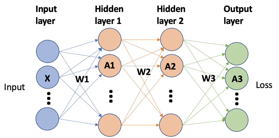
In this example, we have the following computations for forward and backward pass assuming linear layers with ReLU activations. The “@”-symbols denote matrix multiplications.
|
Operation |
Computation |
FLOP forward |
Computation |
FLOP backward |
| Input | A1=W1@X | 2*#input*#hidden1*#batch | dL/dW1 = δ1@X | 2*#input*#hidden1*#batch |
| ReLU | A1R=ReLU(A1) | #hidden1*#batch | δ1 = dδ1R/dA1 | #hidden1*#batch |
| Derivative |
δ1R=dL/dA2 =W2@δ2 |
2*#hidden1*#hidden2*#batch | ||
| Hidden1 | A2=W2@A1R | 2*#hidden1*#hidden2*#batch |
dL/dW2 =δ2@A1R |
2*#hidden1*#hidden2*#batch |
| ReLU | A2R=ReLU(A2) | #hidden2*#batch | δ2 = dδ2R/dA2 | #hidden2*#batch |
| Derivative | δ2R=dL/dA3 =W3@δ3 | 2*#hidden2*#output*#batch | ||
| Hidden2 | A3=W3@A2R | 2*#hidden2*#output*#batch | dL/dW3 =δ3@A2R | 2*#hidden2*#output*#batch |
| ReLU | A3R=ReLU(A3) | #output*#batch | δ3 = dδ3R/dA3 | #output*#batch |
| Loss | L=loss(A3R,Y) | #output*#batch | δ3R = dL/dA3R | #output*#batch |
| Update | W+=lr*δW | 2*#weights |
We separate the weight update from the individual layers since the update is done after aggregation, i.e. we first add all gradients coming from different batches and then multiply with the learning rate.
From this table we see
- ReLUs and the loss function contribute a negligible amount of FLOP compared to layers.
- For the first layer, the backward-forward FLOP ratio is 1:1
- For all other layers, the backward-forward FLOP ratio is 2:1 (ignoring ReLUs)
In equation form, the formula for the backward-forward FLOP ratio is:
backward / forward =
(FIRST LAYER FORWARD FLOP + 2*OTHER LAYERS FORWARD FLOP + WEIGHT UPDATE) / (FIRST LAYER FORWARD FLOP + OTHER LAYERS FORWARD FLOP)
There are two considerations to see which terms dominate in this equation:
- How much of the computation happens in the first layer?
- How many operations does the weight update take compared to the computation in the layers? If the batch size is large or many parameters are shared, this term can be dismissed. Otherwise, it can be approximated as WEIGHT UPDATE ≈ FIRST LAYER FORWARD FLOP + OTHER LAYERS FORWARD FLOP.
This leads us to four possible cases:
|
Big weight update |
Small weight update |
|
|
First layer dominant |
2*FIRST LAYER FORWARD FLOP / FIRST LAYER FORWARD FLOP = 2:1 |
FIRST LAYER FORWARD FLOP / FIRST LAYER FORWARD FLOP = 1:1 |
|
Other layers dominant |
3*OTHER LAYERS FORWARD FLOP / OTHER LAYERS FORWARD FLOP = 3:1 |
2*OTHER LAYERS FORWARD FLOP / OTHER LAYERS FORWARD FLOP = 2:1 |
The norm in modern machine learning is deep networks with large batch sizes, where our analysis predicts a ratio close to 2:1.
In short, our theoretical analysis predicts that the backward-forward FLOP ratio will be between 1:1 and 3:1, with 2:1 being the typical case.
Empirical results
To corroborate our analysis we use NVIDIA’s pyprof profiler to audit the amount of FLOP in each layer during the backward and forward pass.
In this section we will explore:
- The difference between the backward-forward ratio in the first and the rest of the layers.
- The difference between the weight update in convolutional and linear layers.
- The effect of a large batch size on the weight update.
- The effect of depth on the backward-forward ratio.
- The combined effects of batch-size, convolutional layers and depth.
In short, our empirical results confirm our theoretical findings.
In a previous post, we tried to estimate utilization rates. As detailed in the previous post, the profiler does under- and overcounting. Thus, we believe some of the estimates are slightly off.
We have tried to correct them as much as possible. In particular, we eliminate some operations which we believe are double-counted, and we add the operations corresponding to multiplication by the learning rate which we believe are not counted in stochastic gradient descent.
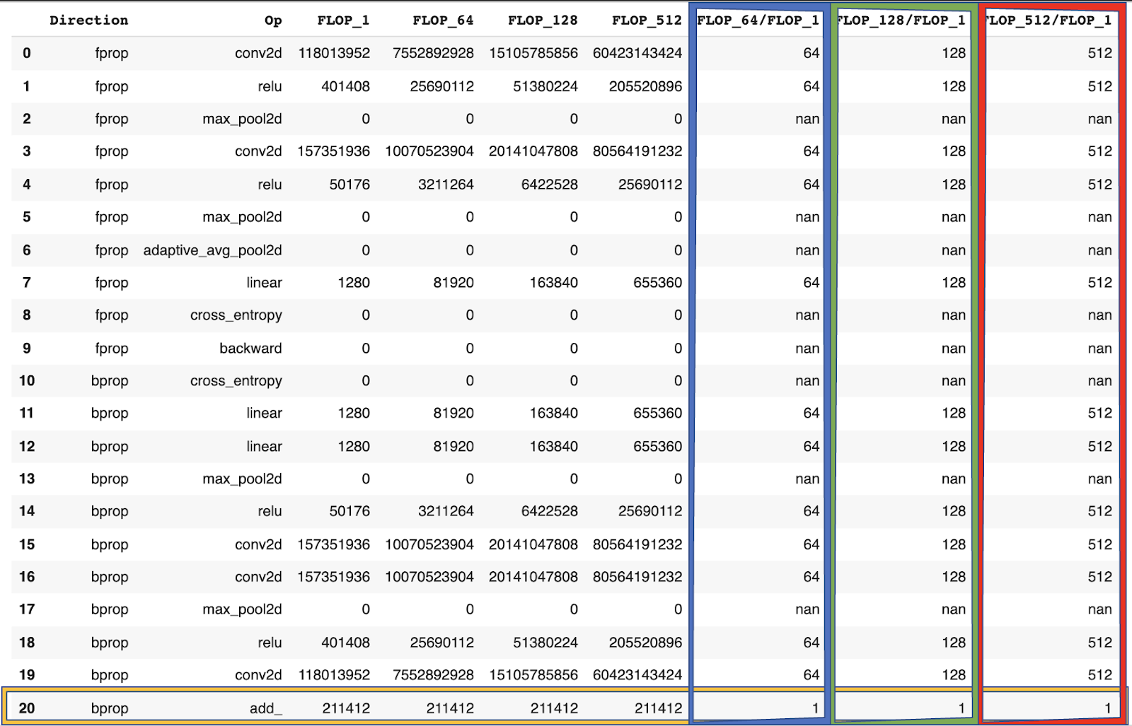
Backward and forward FLOP in the first and the rest of the layers
We can investigate this empirically by looking at a simple linear network (code in appendix).
It results in the following FLOP counts:
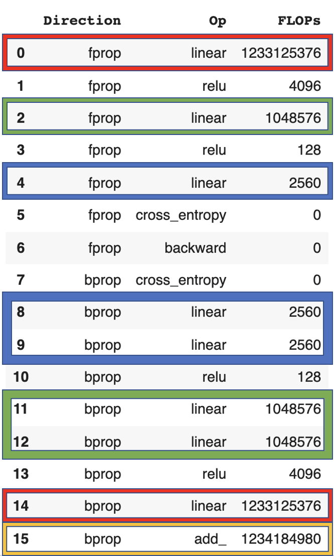
We can see that the first layer (red) has the same flop count for forward and backward pass while the other layers (blue, green) have a ratio of 2:1. The final weight update (yellow) is 2x the number of parameters of the network.
Type of layer
The number of FLOP is different for different types of layers.
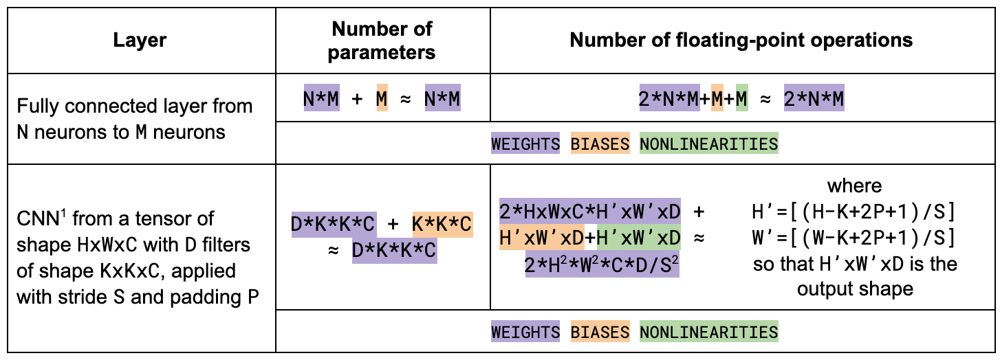
As we can see, the number of FLOP for linear layers is 2x their number of parameters. For CNNs the number of FLOP is much higher than the number of parameters. This means that the final weight update is basically negligible for CNNs but relevant for linear networks.
To show this empirically, we look at the profiler FLOP counts of a small CNN (code in appendix).
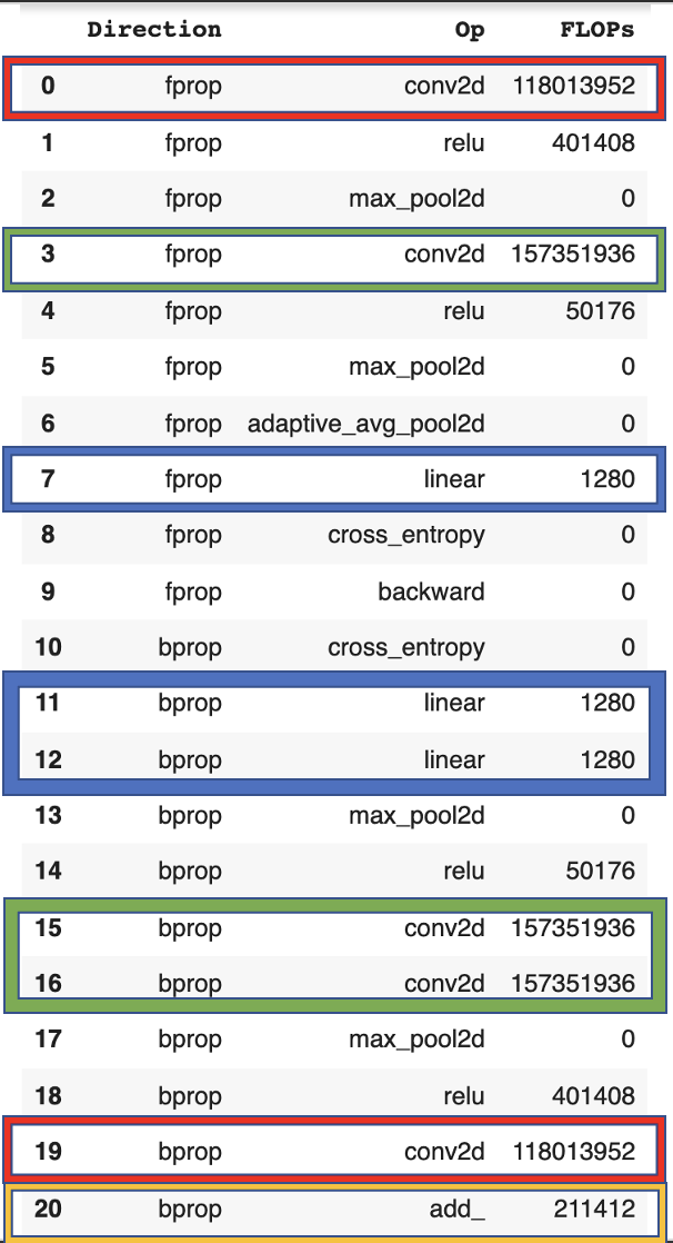
Similar to the linear network, we can confirm that the backward-forward ratio for the first layer is 1:1 and that of all others 2:1. However, the number of FLOP in layers (red, blue, green) is much larger than for the weight update (yellow).
Batch size
Gradients are aggregated before the weight update. Thus, the FLOP for weight updates stays the same for different batch sizes (yellow) while the FLOP for all other operations scales with the batch size (blue, green, red). As a consequence, larger batch sizes make the FLOP from weight updates negligibly small.
Depth
Depth, i.e. the number of layers only has an indirect influence. This stems from the fact that the first layer has a ratio of 1:1 while further layers have a ratio of 2:1. Thus, the true influence comes from FLOP in the first layer vs. every other layer.
To show this effect, we define a CNN with different numbers of intermediate conv layers (code in appendix).
We find that the backward-forward starts significantly below 2:1 for 0 intermediate layers and converges towards 2:1 when increasing the number of intermediate layers.
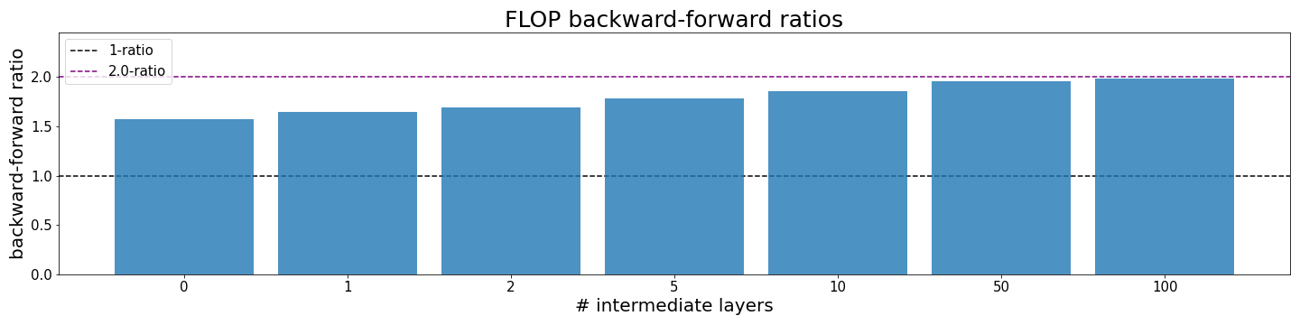
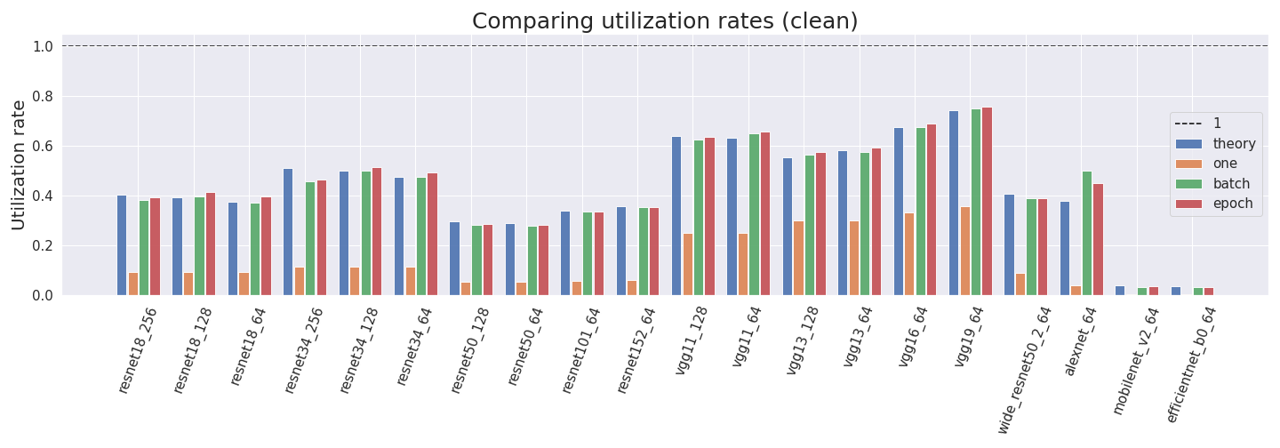
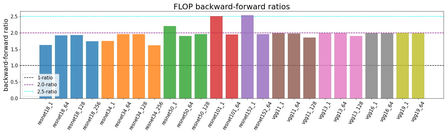
Most common deep learning CNN architectures are deep enough that the first layer shouldn’t have a strong effect on the overall number of FLOP and thus the ratio should be close to 2:1. We have empirically tested this for multiple different types of resnets and batch sizes. We observe some diverge from the expected 2:1 ratio but we think that this is a result of the profiler undercounting certain operations. We have described problems with the profiler in the previous post.

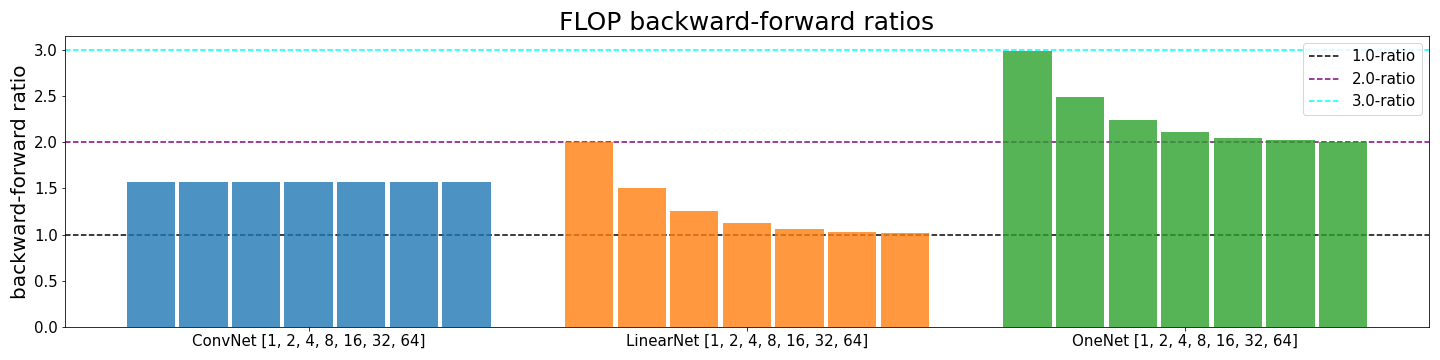
Combining all above
There are interdependencies of batch size, type of layer and depth which we want to explore in the following. We compare the small CNN and the linear network that were already used before with a network we call OneNet (code in appendix). OneNet has only one input neuron and a larger second and third layer. Thus, the ratio between the first and other layers is very small and we can see that the theoretical maximum for the backward-forward ratio of 3:1 can be observed in practice.
Furthermore, we look at exponentially increasing batch sizes for all three architectures. In the case of linear networks, i.e. LinearNet and OneNet, the ratio decreases with increasing batch size since the influence of the weight update is reduced. In the case of the CNN, the FLOP count is completely dominated by layers and the weight update is negligible. This effect is so strong that no change can be observed in the figure.
We see that LinearNet converges to a backward-forward ratio of 1:1 for larger batch sizes while OneNet converges to 2:1. This is because nearly all weights of LinearNet are in the first layer and nearly all weights of OneNet in the other layers.
Conclusion
We have reasoned that the backward-forward FLOP ratio in Neural Networks will typically be between 1:1 and 3:1, and most often close to 2:1.
The ratio depends on the batch size, how much computation happens in the first layer versus the others, the degree of parameter sharing and the batch size.
We have confirmed this in practice. However, we have used a profiler with some problems, so we cannot completely rule out a mistake.
Acknowledgment
The experiments have been conducted by Marius Hobbhahn. The text was written by Marius Hobbhahn and Jaime Sevilla.
Lennart Heim helped greatly with discussion and support. We also thank Danny Hernandez and Girish Sastry for discussion.
Appendix A: Code for all networks
### linear network with large first layer and small later layers
class LinearNet(nn.Module):
    def __init__(self):
        super().__init__()
        self.fc1 = nn.Linear(224*224*3, 4096)
        self.fc2 = nn.Linear(4096, 128)
        self.fc3 = nn.Linear(128, 10)

    def forward(self, x):
        x = torch.flatten(x, 1) # flatten all dimensions except batch
        x = F.relu(self.fc1(x))
        x = F.relu(self.fc2(x))
        x = self.fc3(x)
        return x

### linear network with just one input but larger intermediate layers
class OneNet(nn.Module):
    def __init__(self):
        super().__init__()
        self.fc1 = nn.Linear(1, 4096)
        self.fc2 = nn.Linear(4096, 128)
        self.fc3 = nn.Linear(128, 10)

    def forward(self, x):
        x = torch.flatten(x, 1) # flatten all dimensions except batch
        x = F.relu(self.fc1(x))
        x = F.relu(self.fc2(x))
        x = self.fc3(x)
        return x

### small conv net
class ConvNet(nn.Module):

    def __init__(self):
        super(ConvNet, self).__init__()
        self.conv1 = nn.Conv2d(3, 32, kernel_size=7, stride=2, padding=3, bias=False)
        self.relu = nn.ReLU(inplace=True)
        self.maxpool = nn.MaxPool2d(kernel_size=3, stride=2, padding=1)
        self.conv2 = nn.Conv2d(32, 64, kernel_size=7, stride=2, padding=3, bias=False)
        self.avgpool = nn.AdaptiveAvgPool2d((1, 1))
        self.fc1 = nn.Linear(64, 10)

    def forward(self, x):
        x = self.maxpool(self.relu(self.conv1(x)))
        x = self.maxpool(self.relu(self.conv2(x)))
        x = self.avgpool(x)
        x = torch.flatten(x, 1) # flatten all dimensions except batch
        x = self.fc1(x)
        return x

### conv net with different sizes for intermediate layers
class DeeperConvNet(nn.Module):

    def __init__(self):
        super(DeeperConvNet, self).__init__()
        self.first_layer = nn.Sequential(
            nn.Conv2d(3, 32, kernel_size=7, stride=2, padding=3, bias=False),
            nn.ReLU(inplace=True),
            nn.MaxPool2d(kernel_size=3, stride=2)
        )
        self.conv_layer = nn.Sequential(
            nn.Conv2d(32, 32, kernel_size=3, stride=1, padding=1, bias=False),
            nn.ReLU(inplace=True)
        )
        self.relu = nn.ReLU(inplace=True)
        self.maxpool = nn.MaxPool2d(kernel_size=3, stride=2, padding=1)
        self.convN = nn.Conv2d(32, 64, kernel_size=7, stride=2, padding=3, bias=False)
        self.avgpool = nn.AdaptiveAvgPool2d((1, 1))
        self.fc1 = nn.Linear(64, 10)

    def forward(self, x):
        x = self.first_layer(x)
        for i in range(100):
            x = self.conv_layer(x)
        x = self.relu(self.convN(x))
        x = self.avgpool(x)
        x = torch.flatten(x, 1) # flatten all dimensions except batch
        x = self.fc1(x)
        return x
Appendix B: Using other optimizers
Through this post we have assumed stochastic gradient descent (SGD) for the weight update. SGD involves multiplying the gradient by a learning rate and adding the result to the current weights. That is, it requires 2 FLOP per parameter.
Other optimizers require some extra work. For example, consider adaptive moment estimation (Adam). Adam’s parameter update is given by:
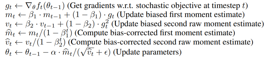
For a total of ~3 + 4 + 3 + 3 + 5 = 18 FLOP per parameter.
In any case, the choice of optimizer affects only the weight update and the amount of FLOP is proportional to the number of parameters. Since batch sizes are typically large, the difference will be small and won’t affect the backward-forward ratio much.
About the authors


Related posts