Optimally Allocating Compute Between Inference and Training
Our analysis indicates that AI labs should spend comparable resources on training and running inference, assuming they can flexibly balance compute between these tasks to maintain model performance.
Published
Resources
Introduction
Sam Altman recently claimed that OpenAI currently generates around 100 billion tokens per day, or about 36 trillion tokens per year. Given that modern language models are trained on the order of 10 trillion tokens and tokens seen during training are around three times more expensive1 compared to tokens seen or generated during inference, a naive analysis2 suggests OpenAI’s annual inference costs are on the same order as their annual model training costs.
This seems like an odd coincidence at first: why should one of these not completely dominate the other? However, there’s a good reason to suppose that these two quantities should be on a similar order of magnitude: the training-inference compute tradeoff. In this post, I will briefly explain what this tradeoff is about and why the current empirical evidence about it implies we should see rough parity in how much compute is spent on training versus inference.
The tradeoff
In general, it’s possible to get a model to perform better by one of two techniques: spending more compute to train the model or spending more compute while running inference with the model. There are a variety of techniques to improve the performance of models at inference time by spending more compute. Some examples for large language models include overtraining the model on a bigger dataset, chain-of-thought prompting, web browsing, and repeated sampling; and for game-playing models based on Monte Carlo Tree Search (MCTS), performing more playouts during runtime is another vital technique for improving performance. A combination of these can allow a smaller model to match the performance of a larger model using less compute during inference.
Villalobos and Atkinson (2023) document the various techniques available for improving performance during inference in the tradeoff table below:
| Technique | Max span of tradeoff in training | Max span of tradeoff in inference | Effect of increasing scale | How current models are used |
|---|---|---|---|---|
| Varying scaling policy | 1.2 OOM | 0.7 OOM | None | Minimal training compute |
| MCTS | 1.6 OOM | 1.6 OOM | Span suddenly approaches 0 as model approaches perfect performance | Mixed |
| Pruning | ~1 OOM | ~1 OOM | Slightly increasing span, increasing returns to training | Minimal training compute |
| Repeated sampling - cheap verification | 3 OOM | 6 OOM | Increasing span | Minimal inference compute |
| Repeated sampling - expensive verification | 1 OOM | 1.45 OOM | None | Minimal inference compute |
| Chain of thought | NA | NA | Unknown | Minimal inference compute |
For example, varying scaling policy means we overtrain models by making their training datasets bigger relative to the compute-optimal dataset scaling rule given by Hoffmann et al. (2022). This gives us some room to reduce the model size without affecting model quality, making inference with the model cheaper as the computational cost of processing a token at short context lengths is proportional to the model size.
Upon considering all of the tradeoffs in the above table, Villalobos and Atkinson (2023) conclude that
Since there is significant variation between techniques and domains, we can’t give precise numbers for how much compute can be traded off in a general case. However, as a rule of thumb, we expect that each technique makes it possible to save around 1 order of magnitude (OOM) of compute in either training or inference, in exchange for increasing the other factor by somewhat more than 1 OOM.
For the sake of simplicity, I will ignore the “somewhat more than” and just focus on the central thesis: approximately, we can spend 1 OOM more on training compute and 1 OOM less on inference, or vice versa, without changing the performance of the resulting model. This tradeoff eventually breaks down, but it seems to hold on a wide range of tasks around the levels of training and inference compute people currently use. In addition, the various techniques from the tradeoff table can often be stacked on top of each other to extend the range in which the training-inference compute tradeoff is possible.
Why we expect investment parity
To see why this implies we should expect the levels of spending on training and inference to be comparable, suppose that a lab was spending 1 zettaFLOP of compute on training and 100 zettaFLOP on inference. Then, they could make use of the training-inference compute tradeoff by increasing their training compute by a factor of 10 and reducing their inference compute by a factor of 10 without affecting the quality of the model from the perspective of users. This new inference setup will give users the same performance, but the lab will be spending \( 10+10 = 20 \; \text{zettaFLOP} \) of compute in total instead of \( 100 + 1 = 101 \; \text{zettaFLOP} \), reducing total costs by a factor of 5. The logic of this simple example generalizes to imply that the setup that minimizes the compute cost of achieving a given level of performance will generally spend the same amount on training and inference.
One concern that we might have is whether this result is unusually sensitive to the magnitude of the tradeoff. What if, instead of 1 OOM (ten times) more training compute allowing us to save 1 OOM of inference compute (i.e. spend ten times less compute on inference), the balance is instead such that it’s enough to spend 0.5 OOMs more training compute to save 1 OOM of inference compute? What does the optimal allocation of compute across training and inference look like in this case?
It turns out the correct strategy when we can trade off \( \beta \) orders of magnitude of training compute for \( \alpha \) orders of magnitude of inference compute is to spend a fraction \( \alpha/(\alpha + \beta) \) on training and a fraction \( \beta/(\alpha + \beta) \) on inference.3 We give a formal proof of this here, but to avoid complexity in the body of the post we instead focus on concrete examples. Suppose we can trade off 1 OOM (ten times) of training compute for 2 OOMs (a hundred times) of inference compute (so \( \beta = 1, \, \alpha = 2 \)) and we have a total of 300 zettaFLOP of compute. If we naively allocate this to training and inference in equal amounts so that each gets 150 zettaFLOP, we will not be acting optimally. This is because if we increase our training compute by 0.1 OOMs and reduce our inference compute by 0.2 OOMs, we’ll leave our performance invariant while changing our total compute use to \( 150 \cdot 10^{0.1} + 150 \cdot 10^{-0.2} \approx 283.4 \; \text{zettaFLOP} \), which is smaller than our compute budget of 300 zettaFLOP. So we’ve reduced our compute expenditure without degrading our performance, showing that our initial allocation was suboptimal.
However, if our allocation is the optimal one of \( (2/3) \cdot 300 = 200 \; \text{zettaFLOP} \) to training and \( (1/3) \cdot 300 = 100 \; \text{zettaFLOP} \) to inference, making the same tradeoff as before changes our total compute from \( 300 \) to \( 200 \cdot 10^{0.1} + 100 \cdot 10^{-0.2} \approx 314.9 \; \text{zettaFLOP} \), which is worse than what we had started with. Indeed, no matter how we change our allocation starting from 200 zettaFLOP to training and 100 zettaFLOP to inference we will not be able to save compute while preserving performance, which is why this particular allocation is efficient.
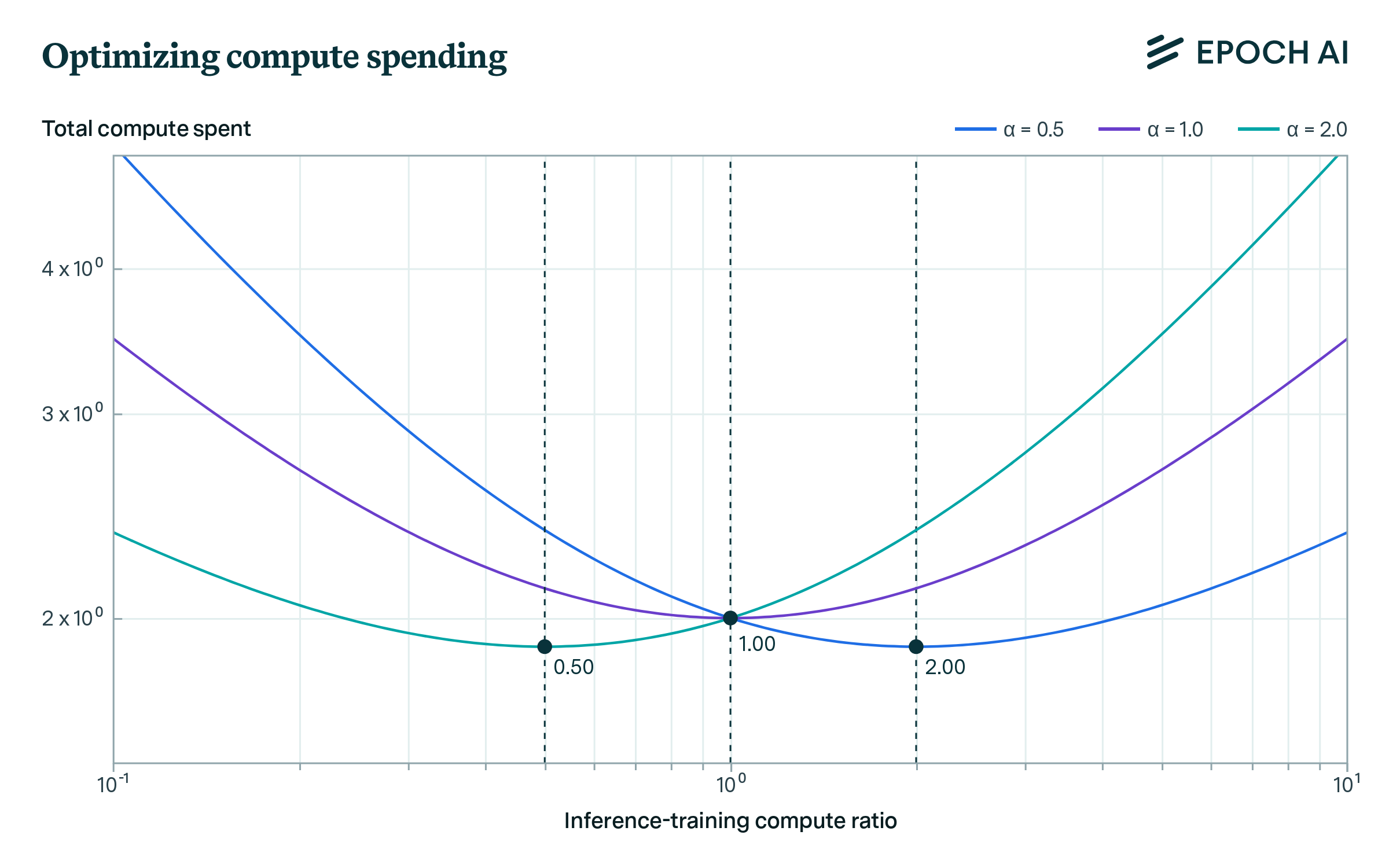
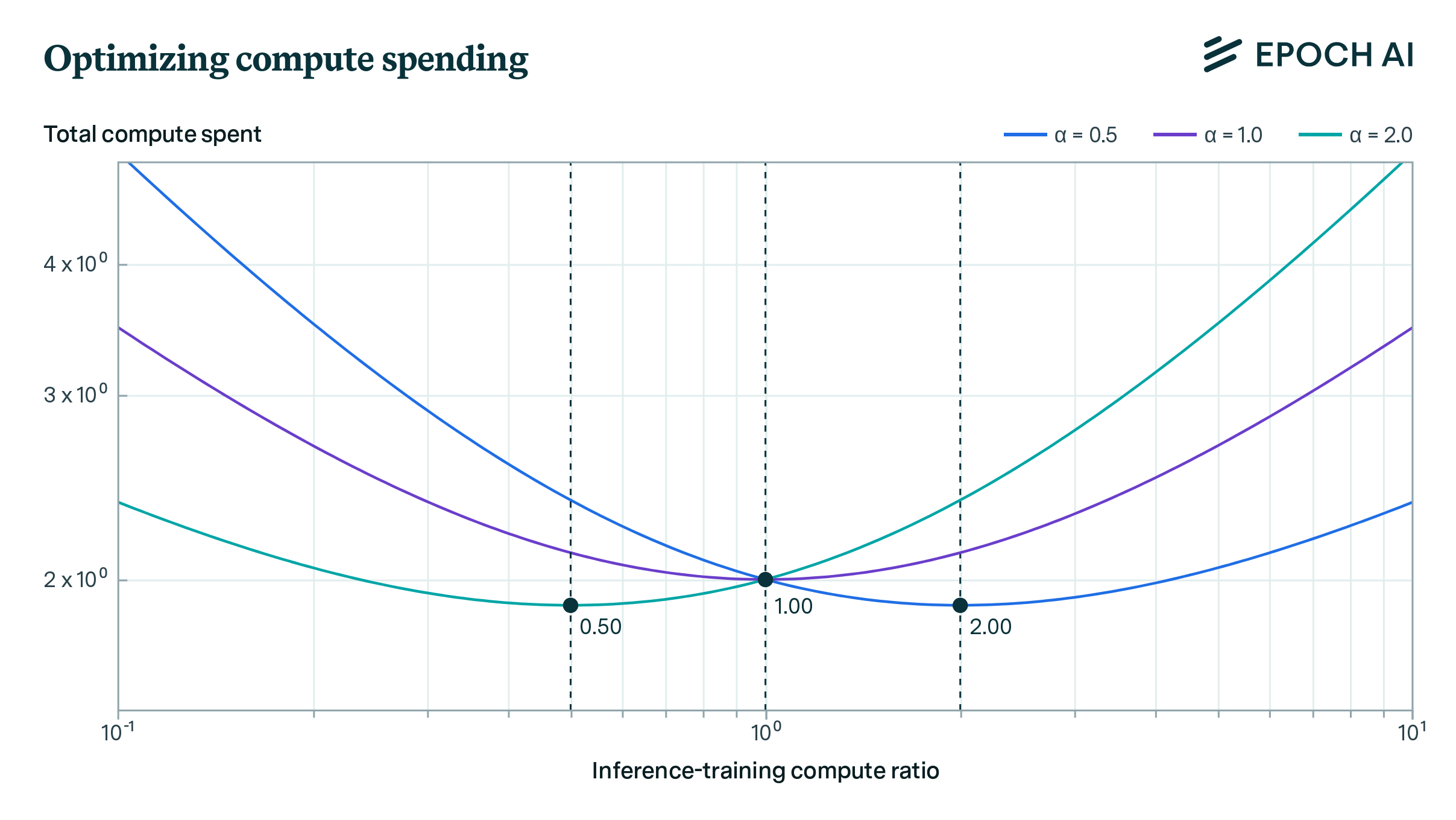
A plot of how total compute spent varies with the inference-training compute ratio for different values of \( \alpha \) assuming \( \beta = 1 \). The optimal values of the ratio for each value of \( \alpha \) are marked in dark grey: they are equal to \( 1/\alpha \) as the above scaling rule suggests.
The main takeaway from this result is if we want training compute and inference compute to not be roughly comparable in magnitude, it’s not enough for \( \alpha \) to be slightly different from 1. Minor deviations of \( \alpha \) from 1 have small effects, and if we want the two compute allocations to be vastly different we’ll need \( \alpha \) to be very far from 1, i.e. less than 0.1 or more than 10 if we want training and inference compute to be of different orders of magnitude. The empirical evidence summarized in the tradeoff table does not support values of \( \alpha \) that are so distant from 1, and this is the primary reason for us to expect compute spent on inference and training to be roughly comparable.
Conclusion
If the training-inference tradeoff holds across a sufficiently wide range of training compute and inference compute values, we should expect similar amounts of computational resources to be spent on training large models and on running inference with them. Phrased differently, we should not expect one of these categories of expenditure to dominate the other by an order of magnitude or more in the future. This result also appears to be robust to plausible uncertainty around the size of the tradeoff, i.e. to how many orders of magnitude of extra training compute we must pay to reduce inference costs by one order of magnitude.
The most plausible way for our conclusion to be wrong is if the known tradeoffs “run out of steam”. For instance, we might be spending most of our compute on inference in a world where we’ve exhausted the gains to be had from all of the inference-saving tradeoffs we know about. If every tradeoff has been adjusted to maximally favor inference and yet inference still dominates the compute cost, there might just be not much more we’re able to do to save on inference costs. On the other hand, there might be other ways of trading off training compute for inference compute that we’re currently not aware of, and the discovery of such ways might extend the range in which the tradeoff is possible. It seems unclear how events will play out on this front.
There are also some less significant factors that we have not considered. For example; inference could face tighter memory bandwidth constraints than training, or more compute could be spent on inference in total because Moore’s law and time discounting ensures compute spent in the future is cheaper than compute spent upfront. In addition, our model assumed that AI developers have perfect foresight about how much demand there will be for their models at particular levels of performance, which is false in practice. These effects are important, but addressing them here would only make the analysis more complicated without changing the basic qualitative result that training and inference compute spending should be in the same ballpark. We intend to build a more realistic model on top of the logic in this post in the future.
Derivation of the optimal scaling policy
Claim: The strategy miniziming total compute expenditure when we can trade off \( \beta \) orders of magnitude of training compute for \( \alpha \) orders of magnitude of inference compute is to spend a fraction \( \alpha/(\alpha + \beta) \) on training and a fraction \( \beta/(\alpha + \beta) \) on inference.
Proof: Suppose we can trade off \( \beta \) orders of magnitude of training compute for \( \alpha \) orders of magnitude of inference compute. Then, if we pick a compute-optimal allocation pair \( (T, I) \) of training compute and inference compute, all of the points \( (10^{-\beta t} T, 10^{\alpha t} I) \) for \( t \in \mathbb R \) will have the same performance from the user’s point of view: they are on the same performance Pareto frontier.
To minimize computational cost while keeping performance the same, we want to minimize the total compute budget \( 10^{-\beta t} T + 10^{\alpha t} I \) with respect to \( t \). If the pair \( (T, I) \) already minimizes total compute \( T + I \) for a fixed performance, which is what we initially assumed, then this sum should attain its minimum value at \( t = 0 \). Differentiating with respect to \( t \) gives \( \alpha \cdot \log(10) \cdot 10^{\alpha t} I - \beta \cdot \log(10) \cdot 10^{\beta t} T \), and setting this to zero at \( t = 0 \) (which is a necessary condition for minimality) gives \( \alpha I = \beta T \). We can therefore see that \( I/(I+T) = \alpha I/(\alpha I + \alpha T) = \beta T/(\beta T + \alpha T) = \beta/(\beta+\alpha) \) and \( T/(T+I) = \alpha/(\beta+\alpha) \), as previously claimed.
Notes
-
When training a model, we need to perform both forward and backward passes, and backward passes are generally twice as expensive to do as forward passes. In contrast, when doing inference, we only need to do forward passes. ↩
-
Ignoring heterogeneity in the models they are using to serve requests and the variance in context lengths across users. ↩
-
Importantly, for this result to hold it’s not necessary for the \( 1:\alpha \) tradeoff to last for many orders of magnitude. As long as the tradeoff appears to hold locally in some neighborhood of the actual choices made by labs, we expect the result to hold with \( \alpha \) equal to the negative of the local elasticity of inference compute with respect to training compute along a performance Pareto frontier. These technical details are not important for the thrust of the argument but they do make the conclusion somewhat more robust than it might appear. ↩
About the authors