Can AI Scaling Continue Through 2030?
We investigate the scalability of AI training runs. We identify electric power, chip manufacturing, data and latency as constraints. We conclude that 2e29 FLOP training runs will likely be feasible by 2030.
Published
Resources
Introduction
In recent years, the capabilities of AI models have significantly improved. Our research suggests that this growth in computational resources accounts for a significant portion of AI performance improvements.1 The consistent and predictable improvements from scaling have led AI labs to aggressively expand the scale of training, with training compute expanding at a rate of approximately 4x per year.
To put this 4x annual growth in AI training compute into perspective, it outpaces even some of the fastest technological expansions in recent history. It surpasses the peak growth rates of mobile phone adoption (2x/year, 1980-1987), solar energy capacity installation (1.5x/year, 2001-2010), and human genome sequencing (3.3x/year, 2008-2015).
Here, we examine whether it is technically feasible for the current rapid pace of AI training scaling—approximately 4x per year—to continue through 2030. We investigate four key factors that might constrain scaling: power availability, chip manufacturing capacity, data scarcity, and the “latency wall”, a fundamental speed limit imposed by unavoidable delays in AI training computations.
Our analysis incorporates the expansion of production capabilities, investment, and technological advancements. This includes, among other factors, examining planned growth in advanced chip packaging facilities, construction of additional power plants, and the geographic spread of data centers to leverage multiple power networks. To account for these changes, we incorporate projections from various public sources: semiconductor foundries’ planned expansions, electricity providers’ capacity growth forecasts, other relevant industry data, and our own research.
We find that training runs of 2e29 FLOP will likely be feasible by the end of this decade. In other words, by 2030 it will be very likely possible to train models that exceed GPT-4 in scale to the same degree that GPT-4 exceeds GPT-2 in scale.2 If pursued, we might see by the end of the decade advances in AI as drastic as the difference between the rudimentary text generation of GPT-2 in 2019 and the sophisticated problem-solving abilities of GPT-4 in 2023.
Whether AI developers will actually pursue this level of scaling depends on their willingness to invest hundreds of billions of dollars in AI expansion over the coming years. While we briefly discuss the economics of AI investment later, a thorough analysis of investment decisions is beyond the scope of this report.
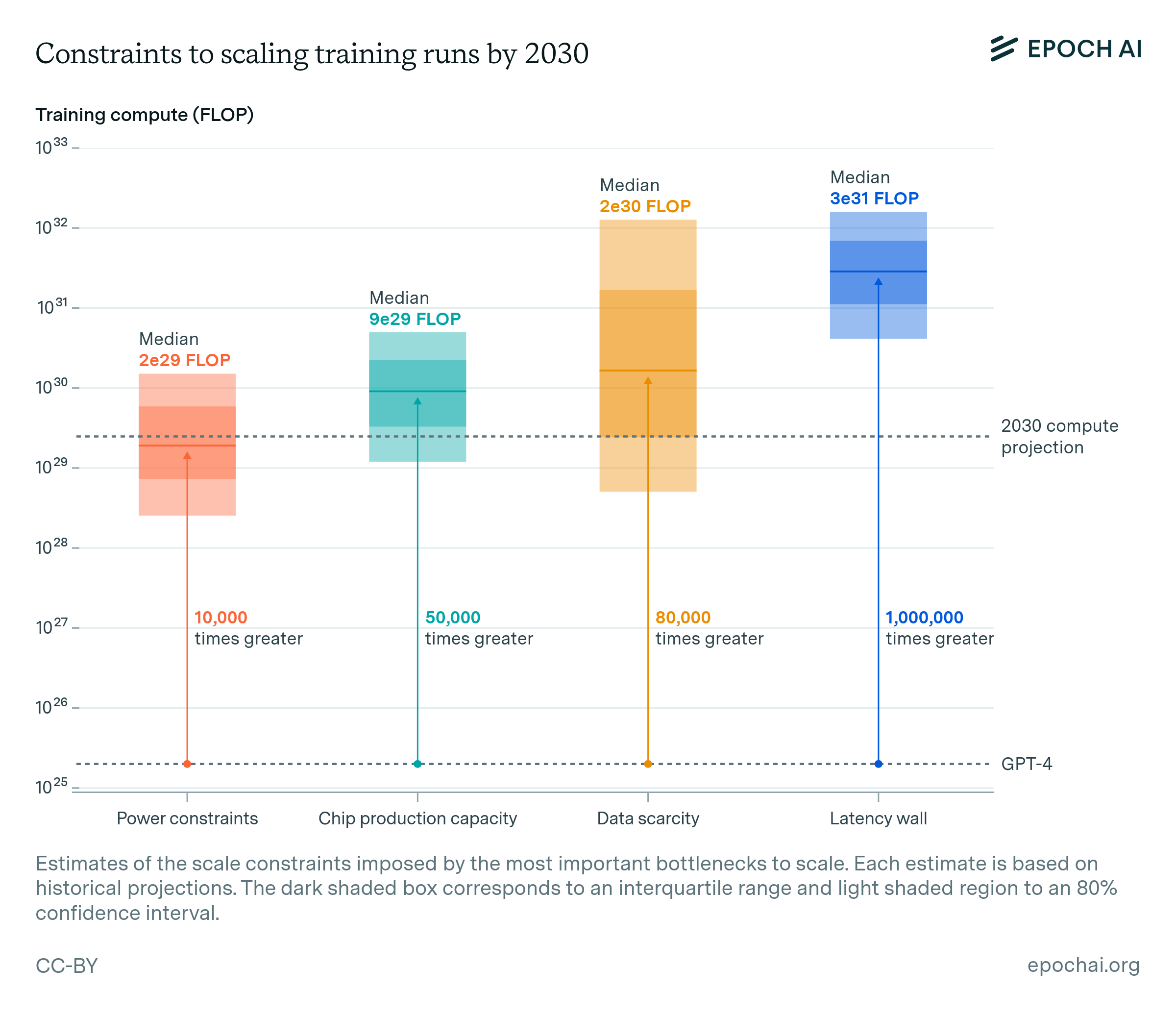
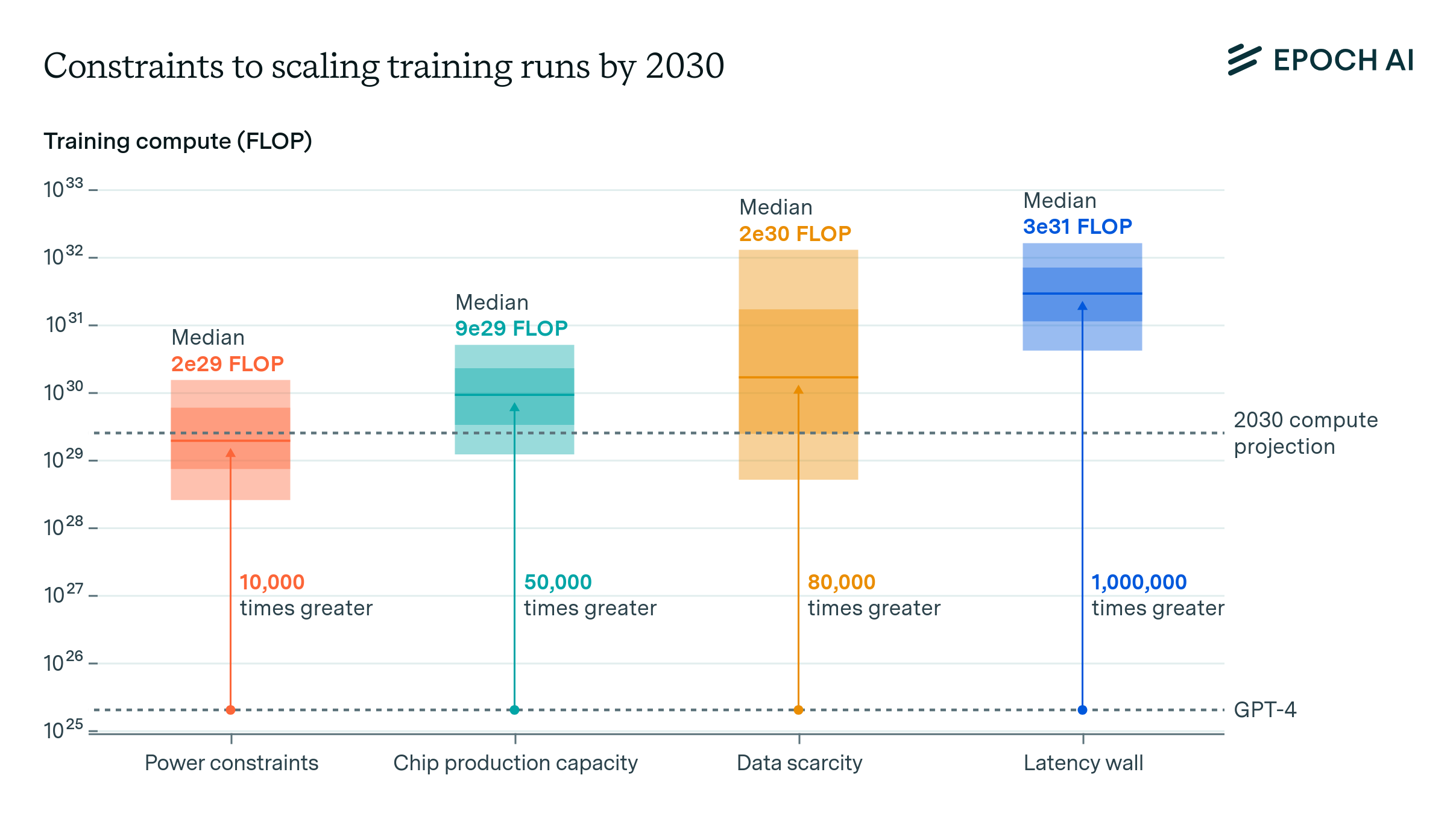
For each bottleneck we offer a conservative estimate of the relevant supply and the largest training run they would allow.3 Throughout our analysis, we assume that training runs could last between two to nine months, reflecting the trend towards longer durations. We also assume that when distributing AI data center power for distributed training and chips companies will only be able to muster about 10% to 40% of the existing supply.4
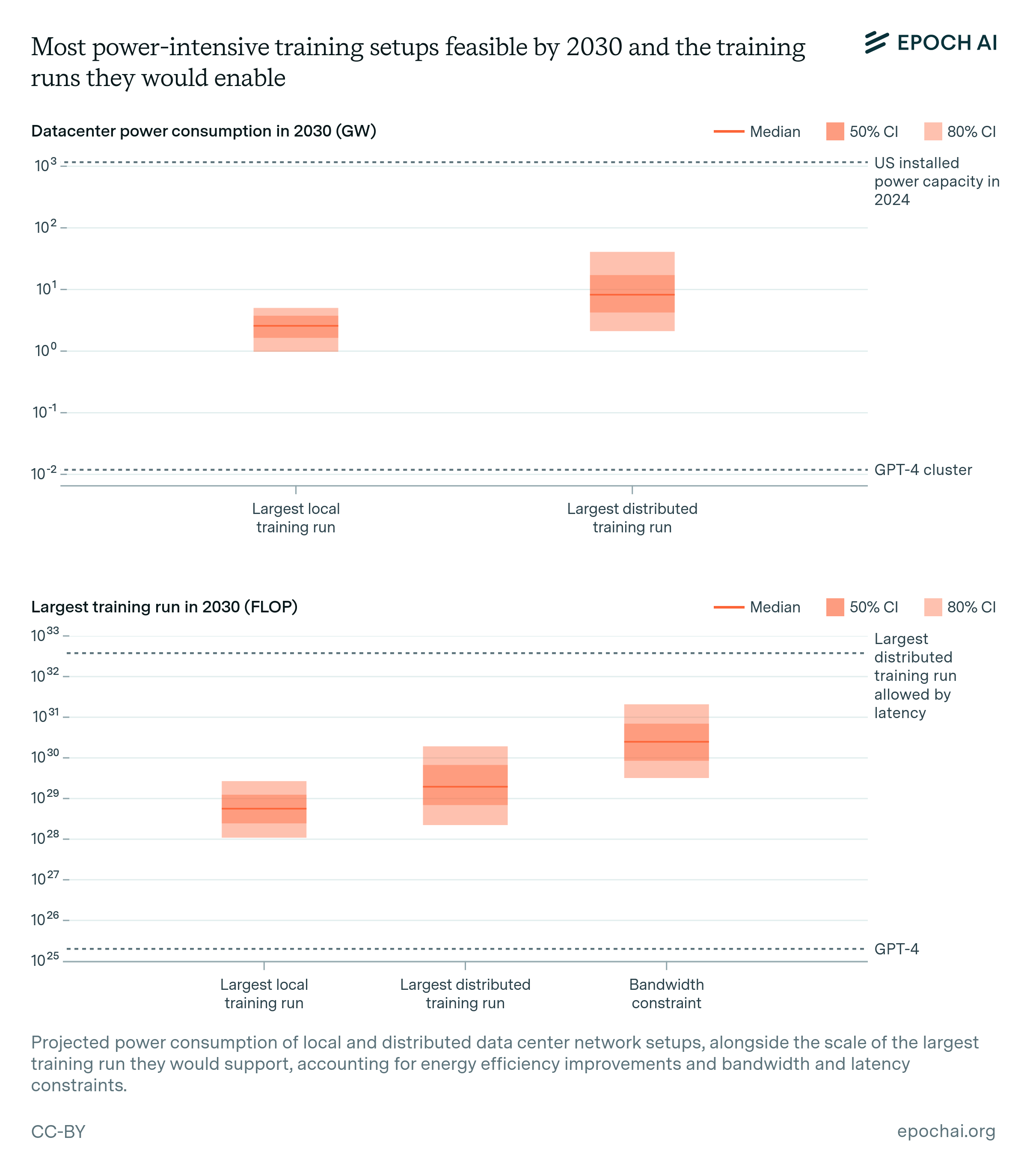
Power constraints. Plans for data center campuses of 1 to 5 GW by 2030 have already been discussed, which would support training runs ranging from 1e28 to 3e29 FLOP (for reference, GPT-4 was likely around 2e25 FLOP). Geographically distributed training could tap into multiple regions’ energy infrastructure to scale further. Given current projections of US data center expansion, a US distributed network could likely accommodate 2 to 45 GW, which assuming sufficient inter-data center bandwidth would support training runs from 2e28 to 2e30 FLOP. Beyond this, an actor willing to pay the costs of new power stations could access significantly more power, if planning 3 to 5 years in advance.
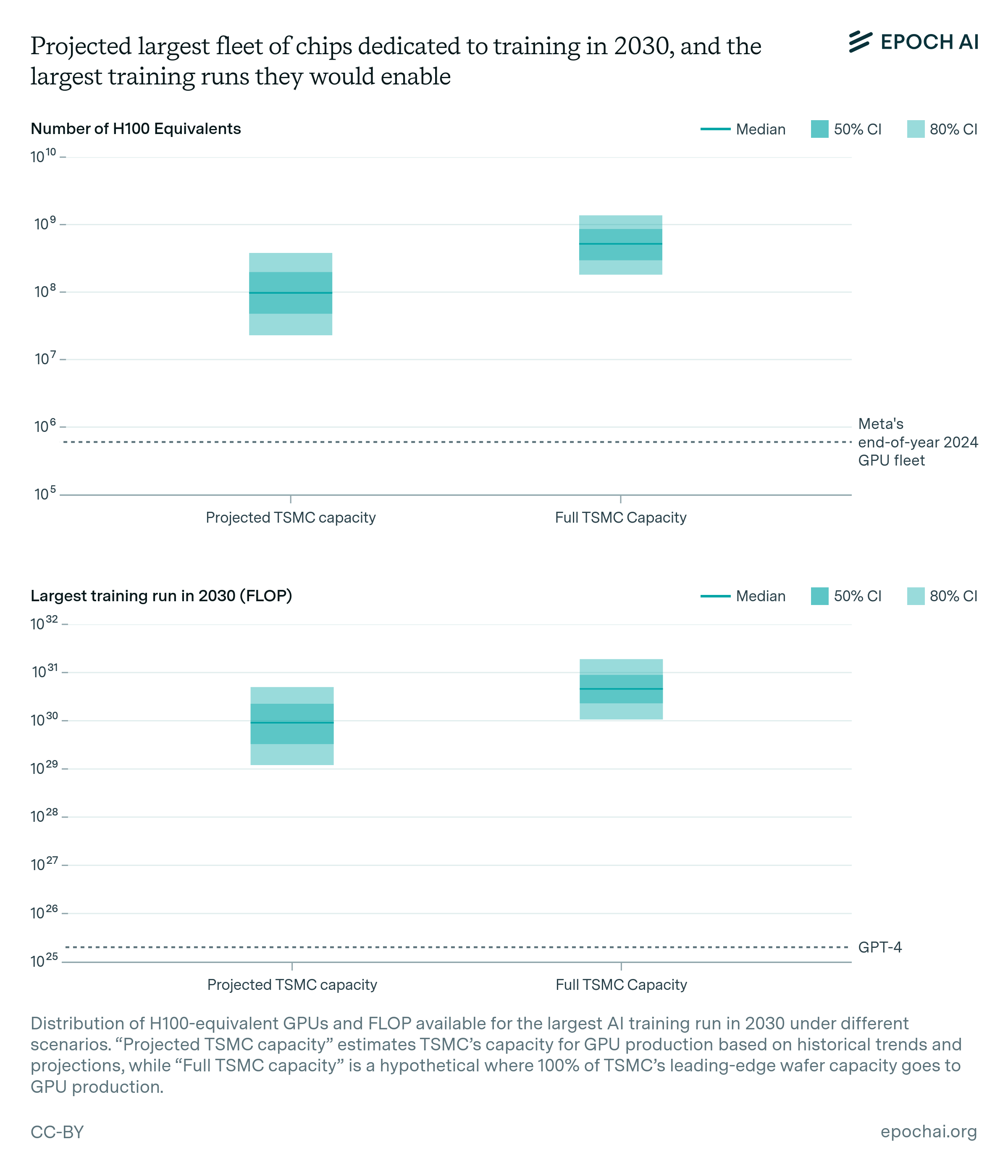
Chip manufacturing capacity. AI chips provide the compute necessary for training large AI models. Currently, expansion is constrained by advanced packaging and high-bandwidth memory production capacity. However, given the scale-ups planned by manufacturers, as well as hardware efficiency improvements, there is likely to be enough capacity for 100M H100-equivalent GPUs to be dedicated to training to power a 9e29 FLOP training run, even after accounting for the fact that GPUs will be split between multiple AI labs, and in part dedicated to serving models. However, this projection carries significant uncertainty, with our estimates ranging from 20 million to 400 million H100 equivalents, corresponding to 1e29 to 5e30 FLOP (5,000 to 300,000 times larger than GPT-4).
Data scarcity. Training large AI models requires correspondingly large datasets. The indexed web contains about 500T words of unique text, and is projected to increase by 50% by 2030. Multimodal learning from image, video and audio data will likely moderately contribute to scaling, plausibly tripling the data available for training. After accounting for uncertainties on data quality, availability, multiple epochs, and multimodal tokenizer efficiency, we estimate the equivalent of 400 trillion to 20 quadrillion tokens available for training by 2030, allowing for 6e28 to 2e32 FLOP training runs. We speculate that synthetic data generation from AI models could increase this substantially.
Latency wall. The latency wall represents a sort of “speed limit” stemming from the minimum time required for forward and backward passes. As models scale, they require more sequential operations to train. Increasing the number of training tokens processed in parallel (the ‘batch size’) can amortize these latencies, but this approach has a limit. Beyond a ‘critical batch size’, further increases in batch size yield diminishing returns in training efficiency, and training larger models requires processing more batches sequentially. This sets an upper bound on training FLOP within a specific timeframe. We estimate that cumulative latency on modern GPU setups would cap training runs at 3e30 to 1e32 FLOP. Surpassing this scale would require alternative network topologies, reduced communication latencies, or more aggressive batch size scaling than currently feasible.
Bottom line. While there is substantial uncertainty about the precise scales of training that are technically feasible, our analysis suggests that training runs of around 2e29 FLOP are likely possible by 2030. This represents a significant increase in scale over current models, similar to the size difference between GPT-2 and GPT-4. The constraint likely to bind first is power, followed by the capacity to manufacture enough chips. Scaling beyond would require vastly expanded energy infrastructure and the construction of new power plants, high-bandwidth networking to connect geographically distributed data centers, and a significant expansion in chip production capacity.
What constrains AI scaling this decade
Power constraints
In this analysis, we project the power requirements necessary to sustain the current trajectory of scaling AI training. We then explore potential strategies to meet these power demands, including on-site power generation, local grid supply, and geographically distributed training networks. Our focus is on AI training runs conducted within the United States, examining the feasibility and constraints of each approach.5
Data center campuses between 1 to 5 gigawatt (GW) are likely possible by 2030. This range spans from Amazon’s 960 MW nuclear power contract in Pennsylvania to the announced 5 GW OpenAI/Microsoft campus. Such campuses would support AI training runs ranging from 1e28 to 3e29 FLOP, given expected advancements in the energy efficiency of ML GPUs.
Scaling beyond single-campus data centers would involve geographically distributed training, which could utilize energy infrastructure across multiple regions. Given current projections, a distributed training network could accommodate a demand of 2 to 45 GW, allowing for training runs of 2e28 to 2e30 FLOP. Bandwidth could also constrain the largest training run that could be done in such a network. Concretely, inter-data center bandwidths of 4 to 20 Petabits per second (Ppbs), which are on trend for existing data centers, would support training runs of 3e29 to 2e31 FLOP. This is likely high enough that bandwidth would not be a major obstacle compared to securing the power supply.6
Larger training runs are plausible: we expect the cost of the infrastructure needed to power GPUs during a training run to be around 40% of the cost of the GPUs themselves by 2030, and rapid expansion of the power supply via natural gas or solar power could be arranged within three to five years of a decision to expand—though this could be constrained by infrastructure-level bottlenecks.
The current trend of AI power demand
AI model training currently consumes a small but rapidly growing portion of total data center power usage. Here, we survey existing estimates of current demand, extrapolates future trends, and compares these projections to overall data center and national power capacity.
Large-scale AI training relies primarily on hardware accelerators, specifically GPUs. The current state-of-the-art GPU is Nvidia’s H100,7 which has a thermal design power (TDP) of 700W. After accounting for supporting hardware such as cluster interconnect and CPUs, and data center-level overhead such as cooling and power distribution, its peak power demand goes up to 1,700W per GPU.8
Using the power demand per GPU, we can estimate the installed power demand for frontier models. The recent Llama 3.1 405B model, with its 4e25 FLOP training run, used a cluster of 16,000 H100 GPUs. This configuration required 27MW of total installed capacity (16,000 GPUs × 1,700W per GPU). While substantial—equivalent to the average yearly consumption of 23,000 US households9—this demand is still small compared to large data centers, which can require hundreds of megawatts.How much will this increase by the end of the decade? Frontier training runs by 2030 are projected to be 5,000x larger than Llama 3.1 405B, reaching 2e29 FLOP.10 However, we don’t expect power demand to scale by as much. This is for several reasons.
First, we expect hardware to become more power-efficient over time. The peak FLOP/s per W achieved by GPUs used for ML training have increased by around 1.28x/year between 2010 and 2024.11 If continued, we would see 4x more efficient training runs by the end of the decade.
Second, we anticipate more efficient hardware usage in future AI training. While Llama 3.1 405B used FP16 format (16-bit precision), there’s growing adoption of FP8 training, as seen with Inflection-2. An Anthropic co-founder has suggested FP8 will become standard practice in frontier labs. We expect that training runs will switch over to 8-bit by 2030, which will be ~2x as power-efficient (e.g. The H100 performs around 2e15 FLOP/s at 8-bit precision, compared to 1e15 FLOP/s at 16-bit precision).12
Third, we expect training runs to be longer. Since 2010, the length of training runs has increased by 20% per year among notable models, which would be on trend to 3x larger training runs by 2030. Larger training run durations would spread out energy needs over time. For context, Llama 3.1 405B was trained over 72 days, while other contemporary models such as GPT-4 are speculated to have been trained over ~100 days. However, we think it’s unlikely that training runs will exceed a year, as labs will wish to adopt better algorithms and training techniques on the order of the timescale at which these provide substantial performance gains.
Given all of the above, we expect training runs in 2030 will be 4x (hardware efficiency) * 2x (FP8) * 3x (increased duration) = 24x more power-efficient than the Llama 3.1 405B training run. Therefore, on-trend 2e29 FLOP training runs in 2030 will require 5,000x (increased scale) / 24x ≈ 200x more power than was used for training of Llama 3.1 405B, for a power demand of 6 GW.
These figures are still relatively small compared to the total installed power capacity of the US, which is around 1,200 GW, or the 477 GW of power that the US produced on average in 2023.13 However, they are substantial compared to the power consumption of all US data centers today, which is around 20 GW,14 most of which is currently not AI related. Furthermore, facilities that consume multiple gigawatts of power are unprecedentedly massive—energy-intensive facilities today such as aluminum smelters demand up to around the order of a gigawatt of power, but not much more.15,16 In the following sections, we investigate whether such energy-intensive facilities will be possible
Power constraints for geographically localized training runs
For geographically localized training, whether done by a single data center or multiple data centers in a single campus, there are two options for supplying power: on-site generation, or drawing from (possibly multiple) power stations through the local electricity grid.
Companies today are already pursuing on-site generation. Meta bought the rights to the power output of a 350MW solar farm in Missouri and a 300MW solar farm in Arizona.17 Amazon owns a data center campus in Pennsylvania with a contract for up to 960 megawatts from the adjoining 2.5 GW nuclear plant. The primary motivation behind these deals is to save on grid connection costs and guarantee a reliable energy supply. In the coming years such data centers might allow unprecedentedly large training runs to take place—960 MW would be over 35x more power than the 27 MW required for today’s frontier training runs.
Could one acquire even more power through on-site generation? Currently, there are at least 27 power plants with capacity greater than 2.5 GW in the US,18 ranging in size up to the Grand Coulee 6.8GW hydroelectric plant in Washington. However, a significant portion of the power capacity from existing plants is likely already committed through long-term contracts.19 This limited availability of spare capacity suggests that existing US power plants may face challenges in accommodating large-scale on-site generation deals. The scarcity of spare energy capacity also breeds disputes. For example, Amazon’s bid for 960 MW of on-site nuclear power is challenged by two utilities seeking to cap Amazon at its current 300 MW purchase. They argue this arrangement evades shared grid costs; such disputes may also inhibit other on-site power deals.
More large-scale plants might be constructed in the coming years, but few have been built recently, and the most recent >3 GW power stations took around five years to build.20 It seems unlikely that any already-planned US power stations will be able to accommodate an on-site data center in the >3 GW range by 2030.21 Instead, moving to larger scales will likely require drawing electricity from the grid.
As a proxy, we can look at data center consumption trends in geographically localized areas. For instance, Northern Virginia is the largest data center hub in the US, housing nearly 300 data centers that are connected to 5 GW of power in peak capacity.22 The largest Northern Virginia electricity provider, Dominion, expects their data center load to increase 4x in the next fifteen years, for an implied 10% yearly growth rate. If Dominion and other regional providers stick to similar expansion plans, by 2030 we might expect data center power capacity in Northern Virginia to grow to around 10 GW.23
Some companies are investigating options for gigawatt-scale data centers, a scale that seems feasible by 2030. This assessment is supported by industry leaders and corroborated by recent media reports. The CEO of NextEra, the largest utility company in the United States, recently stated that while finding a site for a 5-gigawatt AI data center would be challenging, locations capable of supporting 1-gigawatt facilities do exist within the country. It is also consistent with a media report indicating that Microsoft and OpenAI are tentatively planning an AI data center campus for 2028 dubbed Stargate that will require “several gigawatts of power”, with an expansion of up to 5 GW by 2030.24
In sum, current trajectories suggest that AI training facilities capable of accommodating 2 to 5 GW of power demand are feasible by 2030. This assessment is based on three key factors: the projected growth of data center power capacity, exemplified by Northern Virginia’s expected increase from 5 GW to 10 GW; ambitious industry plans for gigawatt-scale data centers, such as the rumored Stargate campus; and utility company assessments indicating that 1 to 5-gigawatt facilities are viable in select US locations. For context, a 5 GW power supply such as the rumored Stargate campus would allow for training runs of 2e29 FLOP by 2030, accounting for expected advances in energy efficiency, and an increase in training duration to over 300 days.25 Training networks powered by co-located power plants or local electricity networks are unlikely to exceed 10 GW—as this would come close to the total projected power demand across all data centers in Northern Virginia.
Power constraints for geographically distributed training
Distributing AI training beyond a single data center can help circumvent local power constraints. Inter-data center distributed training involves spreading workloads across multiple data centers, which may or may not be in close proximity. This method has likely been used for large models like Gemini Ultra, allowing access to more hardware resources.26 Geographically distributed training extends this concept across wider areas, potentially tapping into separate electricity grids. Major tech companies are well-positioned for this approach, with data centers already spread across multiple regions. For example, Google operates data centers in 15 different U.S. states.27 This approach could enable larger-scale training operations by accessing a broader pool of power resources.
How much power could distributed data center networks access? As with local data center networks, we ground our discussion in historical trends, supplier forecasts and third-party projections of data center power growth. In a later section we discuss factors that would affect the feasibility of a major expansion in the US’s overall power supply, which could unlock even more power for data centers.
The potential for US data centers to access electricity is substantial and growing. To accurately assess this capacity, it’s crucial to distinguish between two key metrics: the average rate of actual energy consumption, which accounts for downtime and fluctuations, and the total peak capacity for which data centers are rated. We estimate that average power consumption across US data centers is over 20 GW today.28 Dominion has said that the data centers they serve demand 60% of their capacity on average, and estimates from experts we spoke to suggest that data centers consume around 40-50% of their rated capacity, on average. This suggests an overall capacity of 33 to 50 GW, or ~40 GW as a central estimate.29 In addition, according to SemiAnalysis’ data center industry model, total data center IT capacity in North America (the vast majority of which is in the US) was ~36 GW at the end of 2023 and will be ~48 GW at the end of 2024, which is consistent with this estimate.30
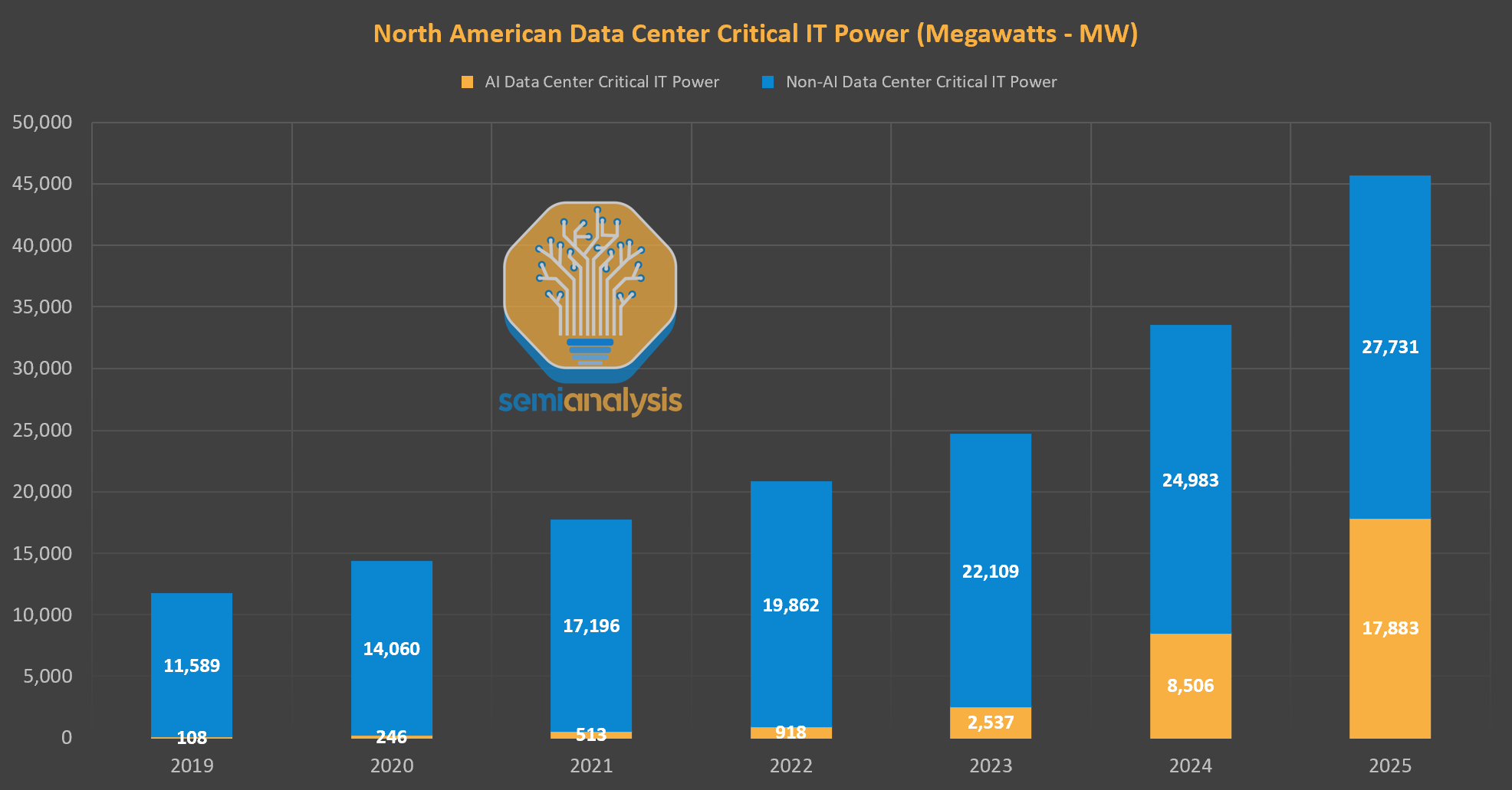
Figure 2: Reported and planned total installed IT capacity of North America data centers via SemiAnalysis’ data center industry model. Important note: to find total capacity, we must multiply these figures by PUE, which ranges from 1.2x for AI datacenters to 1.5x for other datacenters.
The potential for rapid expansion in data center power capacity is significant, as evidenced by multiple sources and projections. Historical data from SemiAnalysis indicates tracked data center capacity grew at an annual rate of ~20% between 2019 and 2023, per (see figure 2). Planned expansions in 2024 and 2025 aim to accelerate this, achieving 32% yearly growth if completed on time.
We can also look at growth projections from utilities companies to estimate a feasible growth rate for the overall data center industry. In Northern Virginia, Dominion is planning for a 10-15% annual growth rate31 in data center power in the coming years, following 24% annual demand growth from 2017 to 2023. NOVEC, another Virginia utility, expects 17% yearly growth in the coming years.
Finally, other independent estimates are consistent with a ~15% annual growth rate, such as from Goldman Sachs, which projects that data center power consumption will grow at an annual rate of 15% to 400 TWh in 2030 (for an average demand of ~46 GW), and from the Electric Power Research Institute (EPRI), which considers a 15% growth rate if there is a rapid expansion of AI applications.
Overall, an annual growth rate of 10-30% seems achievable. A central estimate of 15% growth would imply that US data center capacity could grow from 40 GW to up to 90 GW by 2030, or an increase of 50 GW. Note again that we are using a range of projections of actual growth to ground estimates of feasible growth, so this figure is arguably conservative.
Given power capacity for all data centers, how much power would be available for AI? Currently, the majority of US data centers are dedicated to non-AI uses such as internet services and cloud computing. For instance, SemiAnalysis tracks 3 GW of installed capacity across AI data centers in North America by the end of 2023. This corresponds to ~8% of total data center capacity.32 However, the share of power demand from AI data centers is on the rise, and we expect the AI power capacity share to become even larger in the coming years.
Existing forecasts of the annual growth in power demand for non-AI data centers center around 8% to 11%.33 At a 8% growth rate, demand for non-AI applications would increase from around 37 GW today to around 60 GW by 2030, leaving 90 GW - 60 GW ≈ 30 GW capacity for AI data centers. This would result in roughly a 30 GW / 3 GW ≈ 10x expansion in AI installed capacity, or roughly 47% annual growth on AI installed power capacity.34 This projection assumes a fixed allocation of growth to non-AI applications. However, if AI applications prove more profitable or strategically important, cloud providers could potentially reallocate resources, leading to even higher growth in AI installed power capacity at the expense of non-AI expansion.
Finally, we estimate how much of this capacity can be dedicated to a single training run. We must account for the fact that this added power capacity will likely be shared between different actors, such as Microsoft, Google, Amazon and so on. Our best guess is that the company with the largest share might get around 33% of the power capacity for AI data centers. Companies can front-load their capacity for training, leading to most of their capacity at the time of starting a large training run to be dedicated to training, perhaps by as much as 80%. In total, this means that 33% x 80% = 26% of the AI data center capacity might be used in a single training run.35
Given our estimates, the most well-resourced AI company in the US will likely be able to orchestrate a 30 GW x 26% ≈ 8 GW distributed training run by 2030. After accounting for uncertainties on the relevant growth rates and current capacities, we end up with a conservative estimate of 2 to 45 GW for the largest supply that a developer will be able to muster for distributed training, which would allow for training runs between 2e28 to 2e30 FLOP (see figure 3 in a later section). For context, our earlier analysis suggested that single-campus facilities might achieve 2 to 5 GW capacity by 2030. The upper end of our distributed training estimate (45 GW) significantly exceeds this single-campus projection, indicating the potential for distributed training to overcome power bottlenecks.
Feasibility of geographically distributed training
Geographically distributed training runs, which spread workloads across multiple data centers to alleviate power constraints, are likely to be technically feasible at the scale projected in our analysis. This approach builds upon existing practices in AI model training, where computations are already massively parallelized across numerous GPUs. The fundamental structure of AI training facilitates geographical distribution: datasets are divided into batches, with model weight updates occurring only once per batch. In a distributed setup, these batches can be split across various locations, requiring data centers to synchronize and share gradient updates only at the conclusion of each batch.
Evidence for the viability of this approach exists in current practices. For instance, Google’s Gemini Ultra model was reportedly trained across multiple data centers, demonstrating the practicality of geographically dispersed training.36 While the exact geographic spread of the data centers used for Gemini Ultra is unclear, its training provides a concrete example of large-scale distributed operations.
The feasibility of widely dispersed data centers in distributed training is constrained by latency. In a scenario where major U.S. data centers are connected by an 11,000 km fiber optic loop (a high-end estimate), the communication latency would be approximately 55ms.37 Synchronization would require two round trips down the network, taking 110ms. This is using a travel speed that is two-thirds the speed of light, so this latency cannot be reduced as long as we are doing fiber optic communication. So if a training run is completed within 300 days, it could involve at most 300 days / 110ms = 240 million gradient updates.
We are uncertain how large batches can be without compromising training effectiveness. We will assume it to be 60 million tokens—which is speculated to match the largest batch size achieved by GPT-4 during training. This would allow for ~1e16 tokens (240M batches x 60M tokens/batch) to be seen during training, which under Chinchilla-optimal scaling would allow for a ~6e31 FLOP training run.38 In other words, latency is not likely to be the binding constraint, even when pessimistically assuming a data center network involving very distant data centers.
Beyond latency, bandwidth also influences the feasibility of large-scale distributed training. Current data center switch technology, exemplified by the Marvell Teralynx 10, provides insight into achievable bandwidth. This data center switch supports 128 ports of 400 Gps each, for a total bandwidth of 51.2 Tbps.39 Transmitting the gradient updates for a 16T parameter model at 8-bit precision using a standard two-stage ring all-reduce operation would then take 2 x 16T x 8 bit / 51.2 Tbps = 4.9 seconds per trip. Adding 110ms of latency per all-reduce as before, the total time per all-reduce would be 5 seconds in total. Given Chinchilla scaling, this model size would maximize the scale of training that can be accomplished in under 300 days of training, leading to a 3e28 FLOP training run.40
However, achievable bandwidths are likely to be much higher than what can be managed by a single Teralynx 10 ethernet switch. First, links between data centers pairs can be managed by multiple switches and corresponding fibers, achieving much larger bandwidths. For instance, each node in Google’s Stargate network featured 32 switches managing external traffic. In a ring all-reduce setup, a 32-switch data center could dedicate 16 switches to manage the connection with each of its two neighbors. Given the precedent of Google’s B4 network, we think that switch arrangements of 8 to 32 switches per data center pair should be achievable.41
Second, better switches and transceivers will likely exist in the future, increasing the achievable bandwidth. The broader trend of ASIC switches suggests a 1.4 to 1.6x/year increase in bandwidth,42 which would result in 380 to 850 Tbps ethernet switches by the end of the decade.43
Our final estimate of the achievable inter data center bandwidth by 2030 is 4 to 20 Pbps, which would allow for training runs of 3e29 to 2e31 FLOP. In light of this, bandwidth is unlikely to be a major constraint for a distributed training run compared to achieving the necessary power supply in the first place.
Expanding bandwidth capacity for distributed training networks presents a relatively straightforward engineering challenge, achievable through the deployment of additional fiber pairs between data centers. In the context of AI training runs potentially costing hundreds of billions of dollars, the financial investment required for such bandwidth expansion appears comparatively modest.44
Modeling energy bottlenecks
We conclude that training runs in 2030 supported by a local power supply could likely involve 1 to 5 GW and reach 1e28 to 3e29 FLOP by 2030. Meanwhile, geographically distributed training runs could amass a supply of 2 to 45 GW and achieve 4 to 20 Pbps connections between data center pairs, allowing for training runs of 2e28 to 2e30 FLOP.45 All in all, it seems likely that training runs between 2e28 to 2e30 FLOP will be possible by 2030.46 The assumptions behind these estimates can be found in Figure 3 below.
How much further could power supply be scaled?
At this point, it is unclear to us how far power provision for data centers could scale if pursued aggressively. So far, we have grounded our discussion in the existing power supply for data centers as well as growth projections from utilities, and the results of our model reflect these estimates. How could these numbers change if there is an unprecedented investment in growing the power supply?47
Building new power plants seems reasonably affordable and scalable, but there are also important constraints at the grid level (more below). Natural gas and solar plants can be built relatively quickly, in under two years,48 while other types of power, such as nuclear and hydroelectricity, require longer timeframes,49 and there are no full-scale nuclear plants currently in progress in the US.50
How much would it cost to grow the power supply? As a baseline for the cost of expanding power, we can look at the construction and operation costs of a gas power plant.51
A gas power plant is estimated to have an overnight capital cost on the order of $2,500 per kilowatt with 95% carbon capture, or ~$900 without carbon capture, while the operation cost is roughly 4.5 cents per KWh (and around 4 cents more if carbon capture is included52). However, we should note that the estimates with carbon capture are theoretical, as gas with carbon capture has not been deployed at scale. Gas without carbon capture is cheaper but could be more constrained by politics and corporate commitments (more on this below). Meanwhile, data centers pay around $8.7 cents per KWh for electricity. If we assume a 100% premium on top of the operation cost, data centers would pay ~17 cents/KWh for electricity generated by natural gas with carbon capture.
Meanwhile, an H100 GPU requires 1,700W of power and costs ~$30,000, or ~$17,000 per kilowatt. This means that powering a training run that uses H100s with natural gas would require ~$1500-$4000 in capital costs per H100, and ~$2000 in variable costs.53 So if AI developers had to fund the construction of all the power plants required, this would only increase their hardware costs by around ($4000 + $2000) / $30,000 = 20%. However, this becomes worse after accounting for hardware trends, despite improving efficiency. GPUs are becoming more energy efficient in Watt per FLOP/s at a rate of 2x per three years, but they are also becoming more price-performant in FLOP/dollar at a rate of 2x per two years. So in 2030 each dollar spent on GPUs buys 8x more FLOP, requiring 4x less power, for twice as much power per dollar, and the cost of power would be 40% of the cost of GPUs.
Given these figures, the construction of arbitrarily large power supply networks for data centers is affordable, relative to the cost of the required chips, if power can be scaled up at the current marginal price. But at very large scales beyond ~100 GW, it would require unprecedented effort.
Despite AI developers’ potential willingness to invest heavily in solving power bottlenecks, several obstacles may limit the amount of power available for AI training. Transmission lines, essential for connecting power plants to data centers, typically take about 10 years to complete and often face political challenges. The process of connecting new power generation to the grid, known as interconnection, has become increasingly time-consuming, with average queue durations in the US recently reaching five years.54 Additionally, new electrical transformers, crucial for power distribution, can take up to two years to be delivered. These grid-level bottlenecks create uncertainty about the ability to scale up power supply significantly faster than historical growth rates or the most aggressive utility projections, even with substantial financial investments. The long lead times and complex infrastructure requirements make rapid expansion of power capacity challenging, potentially constraining the growth of large-scale AI training operations.
Another potential constraint is political and regulatory constraints blocking or delaying the construction of power plants, as well as supporting infrastructure such as transmission lines and natural gas pipelines. This could limit or slow down a large scale-up of power. This political constraint may be malleable,55 especially if there is much government support for facilitating the power infrastructure to support development of advanced AI systems.
Scaling up AI training power through natural gas presents its own set of challenges. Large yearly expansions of capacity amounting several dozens of gigawatts have precedent in the US. For example, the US installed a net 250 GW of natural gas from 2000 to 2010, averaging 25 GW per year. But this approach would necessitate increased gas drilling and the construction of additional pipelines to transport the gas to power plants. While at least one analysis suggests the US could drill enough gas to power an extra 100 GW for AI training, there are differing opinions on the viability of this approach. For instance, NextEra’s CEO has identified pipeline construction as a potential obstacle, arguing that renewable energy might be a more feasible option for powering AI data centers.
Finally, there is a tension between massive power growth and the US government’s goal of switching to 100% carbon pollution-free energy by 2035, as well as pledges from the three largest cloud compute providers—Google, Microsoft, and Amazon—to become carbon neutral by 2030. This could limit what types of energy sources could be considered56 (though these commitments may not prove to be binding if there is sufficient economic pressure to scale up AI). For instance, fossil fuel plants may need to be equipped with carbon capture to hold to these commitments, and carbon capture has not yet been tested at scale and may not be ready for widespread deployment by 2030. This tension is especially acute for coal. Coal power may be a source of slack in the power supply, since coal plants are running at ~50% capacity, down from ~70% in 2008, despite many being designed to provide reliable “baseload” power.57 However, coal is much more carbon-intensive than gas.
Given these potential bottlenecks, it is unclear to what degree US power supply can be scaled up arbitrarily by 2030 at a cost resembling the current margin. For this reason, we conservatively assume that power supply will not be scaled beyond the levels forecasted by utilities and independent analysts.
Chip manufacturing capacity
AI chips, such as GPUs, provide the compute required to train AI models and are a key input in AI scaling. Growth in GPU clusters has been the main driver of compute growth in the past few years, and higher performance, lower latency, higher memory bandwidth GPUs make it feasible to do ever larger training runs. AI scaling could therefore be constrained by the number of state-of-the-art GPUs that chipmakers can produce.
We model future GPU production and its constraints by analyzing semiconductor industry data, including projected packaging capacity growth, wafer production growth, and capital expenditure on fabrication plants (fabs). Our projections indicate that GPU production through 2030 is expected to expand between 30% to 100% per year, aligning with CoWoS packaging and HBM production growth rates.
In our median projection, we expect enough manufacturing capacity to produce 100 million H100-equivalent GPUs for AI training, sufficient to power a 9e29 FLOP training run. This estimate accounts for GPUs being distributed among multiple AI labs and partially used for model serving. However, this projection has significant uncertainty, primarily due to unknowns in advanced packaging and high-bandwidth memory capacity expansions. Our estimates range from 20 million to 400 million H100 equivalents, potentially enabling training runs between 1e29 and 5e30 FLOP (5,000 to 250,000 times larger than GPT-4).
Current production and projections
Recent years have seen rapid growth in data center GPU sales. Nvidia, which has a dominant market share in AI GPUs, reportedly shipped 3.76 million data center GPUs in 2023, up from 2.64 million units in 2022.58 By the end of 2023, 650,000 Nvidia H100 GPUs were shipped to major tech companies. Projections for 2024 suggest a potential threefold increase in shipments, with expectations of 1.5 to 2 million H100 units shipped. This volume would be sufficient to power a 6e27 FLOP training run.59
However, if we extrapolate the ongoing 4x/year trend in training compute to 2030, we anticipate training runs of around 2e29 FLOP. A training run of this size would require almost 20M H100-equivalent GPUs.60 If we suppose that at most around 20% of total production can be netted by a single AI lab, global manufacturing capacity would need to reach closer to 100M H100-equivalent GPUs by 2030. This far exceeds current production levels and would require a vast expansion of GPU production.61
TSMC, the company that serves as Nvidia’s primary chip fab, faces several challenges in increasing production. One key near-term bottleneck is chip packaging capacity—particularly for TSMC’s Chip-on-wafer-on-Substrate (CoWoS) process, which is Nvidia’s main packaging method for their latest GPUs. This packaging process combines logic units with high-bandwidth memory (HBM) stacks into ready-to-use AI chips. Packaging is difficult to scale up rapidly, as new facilities require complex equipment from many vendors. Constructing these facilities also requires specialized training for personnel. These constraints have limited TSMC’s AI chip output, despite strong demand from customers like Nvidia.
TSMC is directing significant efforts to address this constraint. The company is rapidly increasing its CoWoS packaging capacity from 14,000-15,000 wafers per month in December 2023 to a projected 33,000-35,000 wafers per month by the end of 2024.62 To further expand this capacity, TSMC opened a new fab in 2023, Advanced Backend Fab 6. At full capacity, this fab could process up to 83,000 wafers per month, which would more than double TSMC’s advanced packaging volume.63 TSMC has also announced plans to increase its packaging capacity by 60% annually through 2026. Recent scale-ups of CoWoS capacity have ranged from 30% to 100% annually. If this trend continues, the number of dies of a fixed size that can be produced will likely increase at a similar rate.64,65
The production of HBM chips themselves is another significant constraint on GPU manufacturing. HBM chips are nearly sold out until 2026. While HBM volume is expected to increase 2-3x from 2023 to 2024, much of this growth comes from reallocating capacity from DRAM, which is another class of lower-end memory chips. SK Hynix, the current HBM leader and Nvidia’s main supplier, projects a 60% annual growth in HBM demand in the medium to long-term (likely referring to revenue), while one analyst firm estimates 45% annual growth in production volume from 2023 to 2028.
HBM production and TSMC’s CoWoS packaging capacity, two key constraints in GPU manufacturing, are projected to expand at similar rates in the coming years. Based on TSMC’s announced plans and recent growth trends in CoWoS capacity, which have ranged from 30% to 100% annually, we estimate GPU production will grow at a similar rate in the near term.
Despite the substantial growth in GPU production, wafer production itself is not likely to be the primary limiting factor. Currently, data center GPUs represent only a small portion of TSMC’s total wafer production. Our central estimate of TSMC’s current production capacity for 5nm and 3nm process nodes is 2.2M wafers per year as of early 2024.66 The projected 2 million H100 GPUs for 2024 would only consume about 5% of the 5nm node’s capacity.67 Even with the projected growth rates, it’s unlikely that GPU manufacturing will dominate TSMC’s leading-edge capacity in the immediate future. Instead, the main constraints on expanding GPU production appear to be chip packaging and HBM production.
However, it is plausible that GPU manufacturing could eventually come to dominate TSMC’s leading-edge nodes. There is precedent for such a scenario; in 2023, Apple absorbed around 90% of TSMC’s 3nm production. Given the high profit margins on AI chips, Nvidia could potentially outbid competitors like Apple and Qualcomm for TSMC’s advanced wafer capacity. While we think this is plausible, this scenario is not featured in our mainline analysis.
Modeling GPU production and compute availability
TSMC forecasted AI server demand to grow at 50% annually over the next five years. Given TSMC’s historical 5 percentage point yearly increase in operating margins, which investors expect to continue due to price hikes, we estimate actual GPU volume growth at around 35% per year.68 This is conservative compared to other projections: AMD expects 70% annual growth for data center chips through 2027, implying about 60% annual GPU volume growth assuming similar price increases.69 These more aggressive estimates align closely with near-term CoWoS packaging and HBM production scale-up projections discussed above, lending them credibility. We take this range of estimates into account, and project production of GPU dies to expand somewhere between 30% and 100% per year.
We expect that there will be enough wafer capacity to sustain this expansion. TSMC’s historical trends show capex growth of 15% annually and wafer capacity expansion of 8% yearly from 2014 to 2023.70 TSMC might increase its capex dedicated to expanding GPU production and substantially expand the production of GPU-earmarked-wafers, packaging and other parts of the production. If TSMC accelerates its capex growth to match their expected growth in the AI server market of 50% annual growth, the historical relationship between input and output growth suggests that total wafer capacity could expand by 27% per year.71 Overall, this points to a growth rate of leading-edge wafer production of between 5% and 20% per year.
We have appreciable uncertainty about current leading-edge wafer production, and assume that this is somewhere between 100k to 330k/month. At 5 to 20% yearly growth, we project the total stock of leading-edge wafers produced by 2030 to be between 10M and 37M. Based on TSMC’s and others’ projections, we expect around 20% of these wafers to be dedicated to producing data center GPUs.
These projections indicate that 2e30 to 4e31 FLOP/year worth of global stocks of H100 equivalents will be produced in aggregate. Of course, only some fraction of this will be dedicated to a single training run, since individual labs will only receive some small fraction of shipments, labs will earmark their GPUs to inference and other experiments, and training runs will likely last less than a year. At current rates of improvements in hardware and algorithms and growing budgets for AI, training runs will likely not exceed six months if hardware or software progress does not slow. We assume that training runs will last around 2 to 9 months; on the higher end if progress in hardware and software stalls, and the lower end if progress accelerates relative to today.
It is likely that AI chips will be distributed across many competing labs, with some lab owning some non-trivial fraction of global compute stocks. For instance, Meta reportedly bought one fourth of H100 shipments to major companies in 2023. We estimate that recently, the share of datacenter GPUs owned by a single lab at any point in time might be somewhere between 10% and 40%.
Of this allocation, some fraction will likely be tied up with serving models and unavailable for training. It is difficult to know what fraction this might be. However, we can use a simple heuristic argument. A simple analysis suggests AI labs should allocate comparable resources to both tasks. If this holds, and compute for training continues to grow 4x per year, then we should expect about 80% of the total available compute to be used to train new models.72
Putting all this together leads us to the following picture. On the median trajectory, about 100M H100-equivalents could, in principle, be dedicated to training to power an 9e29 FLOP training run. However, this projection carries significant uncertainty, with our estimates ranging from 20 million to 400 million H100-equivalents, corresponding to 1e29 to 5e30 FLOP. To establish an upper bound, we considered a hypothetical scenario where TSMC’s entire capacity for 5nm and below is devoted to GPU production, from now until 2030. In this case, the potential compute could increase by an order of magnitude, reaching 1e30 to 2e31 FLOP. This upper limit, based on current wafer production projections, illustrates the maximum possible impact on AI training capabilities if existing constraints in packaging, HBM production, and wafer allocation were fully resolved. Figure 4 below illustrates these estimates, and lists the assumptions behind them.
Data scarcity
Scaling up AI training runs requires access to increasingly large datasets. So far, AI labs have relied on web text data to fuel training runs. Since the amount of web data generated year to year grows more slowly than the data used in training, this will not be enough to support indefinite growth. In this section, we summarize our previous work on data scarcity, and expand it by estimating further possible gains in scale enabled by multimodal and synthetic data.
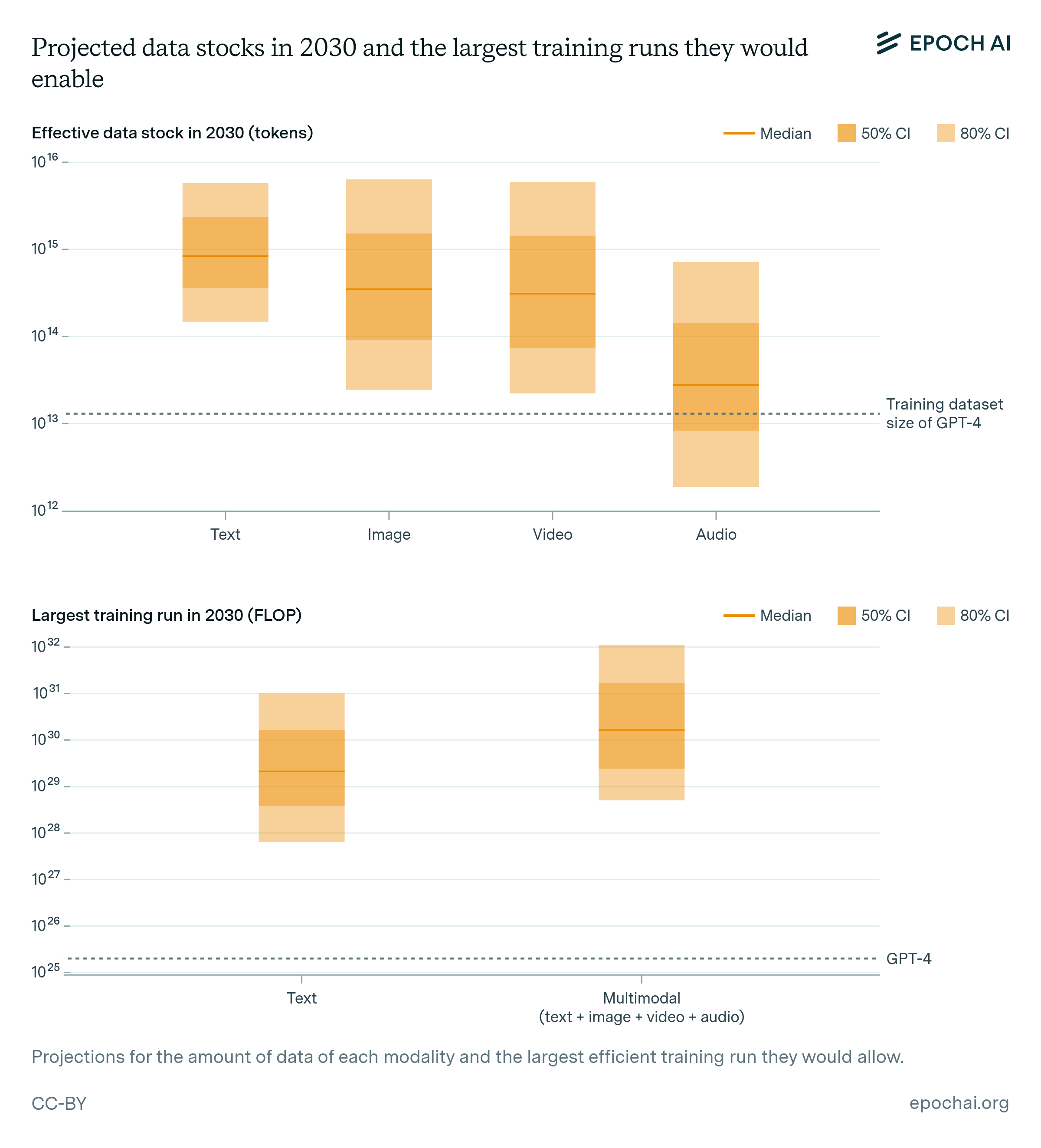
The largest training datasets known to have been used in training are on the order of 15 trillion tokens of publicly available text and code data.73 We estimate that the indexed web contains around 500 trillion tokens after deduplication, 30 times more data than the largest known training datasets. This could be as low as 100T if only looking at already compiled corpora like CommonCrawl, or as high as 3000T if also accounting for private data.74
Since the Chinchilla scaling laws suggest that one ought to scale up dataset size and model size proportionally, scaling up training data by a factor of 30x by using the entirety of the indexed web would enable AI labs to train models with 30x more data and 30x more parameters, resulting in 900x as much compute, i.e. up to 8e28 FLOP if models are trained to be Chinchilla-optimal.75,76,77
If the recent trend of 4x/year compute scaling continues, we would run into this “data wall” for text data in about five years. However, data from other modalities and synthetic data generation might help mitigate this constraint. We will argue that multimodal data will result in effective data stocks of 450 trillion to 23 quadrillion tokens, allowing for training runs of 6e28 to 2e32 FLOP. Furthermore, synthetic data might enable scaling much beyond this if AI labs spend a significant fraction of their compute budgets on data generation.78
Copyright restrictions
Published text data may be subject to copyright restrictions that prohibit its use in training large language models without permission. While this could theoretically limit the supply of training data, several factors mitigate this concern in practice. The primary consideration is the ongoing legal debate surrounding whether the inclusion of published text in a general-purpose model’s training data constitutes “fair use”. However, even if this debate is settled in favor of copyright holders, there are further practical considerations that complicate the enforcement of such restrictions.
Many large repositories of public web data, such as Blogspot, allow individual authors to retain copyright of their content. These individuals, however, may face significant challenges in proving the inclusion of their content in training data and may lack the capacity or desire to engage in complex litigation processes. This practical barrier can prevent individual content creators from pursuing legal action against AI companies using their data.
On the other hand, larger publishers like newspapers typically have the resources to litigate for copyright infringement. However, these entities can also negotiate agreements with AI companies to license their data. For instance, OpenAI has successfully reached agreements with several major publishers, including StackOverflow, The Atlantic, TIME, and Vox Media. These agreements demonstrate that AI companies can often navigate copyright restrictions effectively through negotiation and collaboration with content providers.
Ultimately, the full extent to which copyright restrictions will limit the supply of training data for large language models remains uncertain. While legal and practical challenges exist, it seems unlikely that these constraints will significantly reduce the overall volume of available data. The vast amount of content on the internet, combined with the complexities of enforcement and the potential for licensing agreements, suggests that AI companies will still have access to substantial datasets. However, it’s worth noting that copyright restrictions may disproportionately affect high-quality sources such as books and reputable news outlets. These sources often contain well-curated, factual, and professionally edited content, which could be particularly valuable for training. As a result, while the quantity of training data may not be drastically reduced, there could be a notable impact on the quality and diversity of the most authoritative sources available for AI training.
Multimodality
AI labs could leverage other data modalities such as image or video.79 Current multimodal foundation models are trained on datasets where 10-40% is image data.80 This data is used to allow models to understand and generate images. Given the usefulness of multimodal understanding, we expect future datasets to include a significant portion of non-text data purely for this purpose. That said, to significantly expand the stock of data, the portion of multimodal data would have to become far greater than that of text data.
Audio, image or video modeling will be valuable enough on its own that AI labs will scale pure audiovisual training. Strong visual abilities could enable models to act as assistants embedded within workflows to organize information or operate a web browser. Models that have fluent, fast, multilingual speech abilities are likely to enable much improved personal voice assistant technology, realtime translation, customer service and more fluid interactions compared to text-only. While current vision models use much less compute than language models,81 in a scenario where text data is a bottleneck but image data is plentiful, AI labs might start dedicating more resources to image models.
Additional modalities like protein sequences or medical data are also valuable. However, the stock of such data is unlikely to be large enough to significantly expand the stock of available training data.82
Multimodal data can further aid language understanding in various ways. Textual data can be transcribed from audio, image and video data, which could further expand the stock of text-related data.83 More speculatively, non-text data may improve language capabilities through transfer learning or synergy between modalities. For example, it has been shown that combining speech and text data can lead to improved performance compared to single-modality models, and it is suggested that such synergies improve with scale. However, research on transfer learning between modalities is scarce, so we can’t conclude with certainty that transfer learning from multimodal data will be useful.
How much visual data would be available for training if one of these scenarios came to pass? The internet has around 10 trillion seconds of video, while the number of images may also be close to 10T.84 It’s challenging to establish a rate of equivalence between these modalities and text data. Current multimodal models such as Chameleon-34B encode images as 1024 tokens, but we expect that as multimodal tokenizers and models become more efficient this will decrease over time. There are examples of efficient encoding of images with as few as 32 tokens, which after being adjusted by typical text dictionary size would result in 22 tokens per image.85 We take 22 tokens per image and second of video as a central guess, which means that image and video multimodality would increase the effective stock of data available for training by roughly 400T tokens.86 This suggests that image and video content might each contribute as much as text to enable scaling. This would allow for training runs ten times larger than if trained purely on text data.
Moreover, there are probably on the order of 500B-1T seconds of publicly available audio on the internet.87 Neural encoders can store audio at <1.5 kbps while being competitive with standard codecs at much higher bitrate. This corresponds to <100 language-equivalent tokens per second of audio. So it seems likely that total stored audio is on the order of 50-100T trillion tokens, not far from text and image estimates.88 Hence, this would probably not extend the stock of data by a large factor.
After adding the estimates from all modalities and accounting for uncertainties in the total stock of data, data quality, number of epochs, and tokenizer efficiency, we end up with an estimate of 400 trillion to 20 quadrillion effective tokens available for training, which would allow for training runs of 6e28 to 2e32 FLOP by 2030 (see Figure 5).
Given how wide this interval is, it may be useful to walk through how the high end of the range could be possible. Note that these numbers are merely illustrative, as our actual confidence interval comes from a Monte Carlo simulation based on ranges of values over these parameters.
A high-end estimate of the amount of text data on the indexed web is two quadrillion tokens (Villalobos et al, 2024). Meanwhile, a high-end estimate of the number of images and seconds of video on the internet is 40 trillion. If we also use a higher-end estimate of 100 tokens per image or video-second, this would mean four quadrillion visual tokens, or six quadrillion text and visual tokens. If we also assume that this stock of data doubles by 2030, 80% is removed due to quality-filtering (FineWeb discarded ~85% of tokens), and models are trained on this data for 10 epochs, this would lead to an effective dataset size of ~20 quadrillion tokens. See Figure 5 for a full list of these parameters and our reasoning for the value ranges we chose.
Synthetic data
In our projections we have only considered human-generated data. Could synthetic data generation be used to greatly expand the data supply? Several important milestones in machine learning have been achieved without relying on human data. AlphaZero and AlphaProof learned to play games and solve geometry problems respectively, matching or surpassing human experts by training purely on self-generated data. Language models fine-tuned on synthetic data can improve their ability to code and answer reasoning questions. Small LLMs trained on carefully curated synthetic data can achieve comparable or superior performance with significantly fewer parameters and less training data compared to larger models trained on web-scrape text. Large-scale frontier language models like Llama 3.1 use synthetic data to augment capabilities in areas where collecting high-quality human-annotated data might be challenging or costly, such as long-context capabilities, multilingual performance, and tool use capabilities.
One key reason to expect it should be possible to spend compute to generate high-quality synthetic data is that it’s often easier to verify the quality of an output than it is to generate it. This principle most clearly applies in domains where we can create explicit correctness or quality signals. For example, in coding tasks, we can check if generated code passes unit tests or produces correct outputs for sample inputs. In mathematics, we can detect logical or arithmetic mistakes and correct them.
This process enables developers to use compute to generate numerous candidate solutions. They can then systematically verify the correctness or quality of each generated solution, keeping only the high-quality examples while discarding the subpar ones. This approach can computationally create datasets filled with high-quality, synthetic examples. For these tasks, one can expend more inference compute to generate outputs of higher quality.
The verification-easier-than-generation principle may extend beyond coding to various other domains. For instance, it’s often easier to review a research paper for quality and novelty than to write an original paper. Similarly, evaluating the coherence and plausibility of a story is typically less challenging than writing an engaging story from scratch. In these cases, while traditional symbolic systems might struggle with verification, modern AI systems, particularly large language models, have demonstrated evaluation capabilities comparable with human verifiers. This suggests that AI-driven verification could enable creating high-quality synthetic data in these complex domains.
There are additional mechanisms which can be used to generate high-quality synthetic data. For example, it is often the case that a model cannot produce high-quality outputs directly, but it can produce them by combining several smaller steps. This is the key idea behind chain-of-thought prompting, which can be used to teach models increasingly complex arithmetic by bootstrapping from simpler examples.
Generating endless data
Even if it is technically possible to generate useful synthetic data for a wide range of tasks, the computational overhead of generation might preclude its usage in practice. We can try to estimate how much additional compute would be needed to scale models using synthetic data, compared to a baseline of scaling natural datasets.
Suppose that we have access to a frontier model which we will use as a data generator, and want to train a target model with 10x more compute than the generator. We want the new model to achieve a similar quality than would be obtained by training it on natural data. In previous work, we quantified the extent to which spending more compute at inference time improves the quality of outputs that models can achieve. Concretely, chain-of-thought was found to lead to a compute-equivalent-gain of 10x while increasing inference costs by 10x.
This means that increasing the compute usage of the generator during inference by 10x (by generating outputs step by step) raises the quality of the outputs to the level of a model trained on 10x more compute. We can then train our new model on these high-quality outputs to reach the desired level of performance.
Assuming the new model is trained in a compute-optimal fashion, the computational cost of generating the new training dataset would be similar to the cost of training the new model.89 So using synthetic data would double the compute requirements to train a model, compared to using natural data.
Spending so much compute on synthetic data generation for training would not be unprecedented: DeepMind spent roughly 100x more compute on game simulations to generate data for AlphaGo Zero than in training the underlying model. However, this is very speculative; for example we haven’t yet seen such a technique applied successfully at scale to frontier model pretraining.
There are several obstacles for using synthetic data. The first is the possibility of model collapse: over-reliance on synthetic data might cause a degeneration or stagnation of capabilities. It’s unclear if the self-correction mechanisms we have introduced are enough to avoid this outcome, although there are promising signs.
Increasing compute allocation for data generation can enhance synthetic training data quality through two types of approaches: generating many candidates then filtering for quality, and employing compute-intensive methods like chain-of-thought reasoning to produce superior outputs directly. However, this strategy may face diminishing returns as compute investment grows. When verification or quality estimation processes are imperfect, improvements in data quality may plateau despite additional compute allocation.90
Synthetic data is already useful for domains where verification is straightforward such as math and coding or in a small set of domains where collecting high-quality human-annotated data might be challenging or costly, such as tool use, long-context data or preference data. Based on this success, and the intuitions we’ve discussed, we find it plausible that high-quality synthetic data generation is possible in a wide range of fields, beyond what has been demonstrated until now, but this is still uncertain. In this case, data availability might not pose a constraint on scaling, as more could be generated on demand by spending enough compute.
We expect synthetic data to likely be useful for overcoming data bottlenecks. However, the research on the topic is nascent and the state of existing evidence is mixed, and so in this article we conservatively rely on estimates from multimodal data, excluding all types of synthetic data.
Latency wall
Another potential constraint to AI scaling is latency. There is a minimum time required for a model to process a single datapoint, and this latency grows with the size of the model. Training data is divided into batches, where the data in a batch can be processed in parallel, but there are limits to how large these batches can be. So a training run must last at least as long as the time to process one batch, multiplied by the number of training batches (training dataset size divided by the batch size). Given a finite training run duration, this dynamic limits the size of a model and how much data it can be trained on, and thus the total size of the training run.91
This constraint does not pose much of an issue for today’s training runs because typical latencies are very small. However, it could become substantially more important in larger training runs as the minimum latency increases with model size due to the sequential nature of operations across layers.
Training runs can partially manage this latency issue by increasing the batch size, allowing more data to be processed in parallel. In particular, increasing the batch size improves the convergence of stochastic gradient descent, at the cost of more computational resources. This enables one to speed up training at the cost of more compute per batch size, though without substantially increasing the overall compute needed for training. However, beyond a “critical batch size”, further batch increases yield drastically diminished returns per batch. It is therefore not efficient to scale batches indefinitely, and training a model on ever-larger datasets requires increasing the number of batches that need to be processed in sequence.
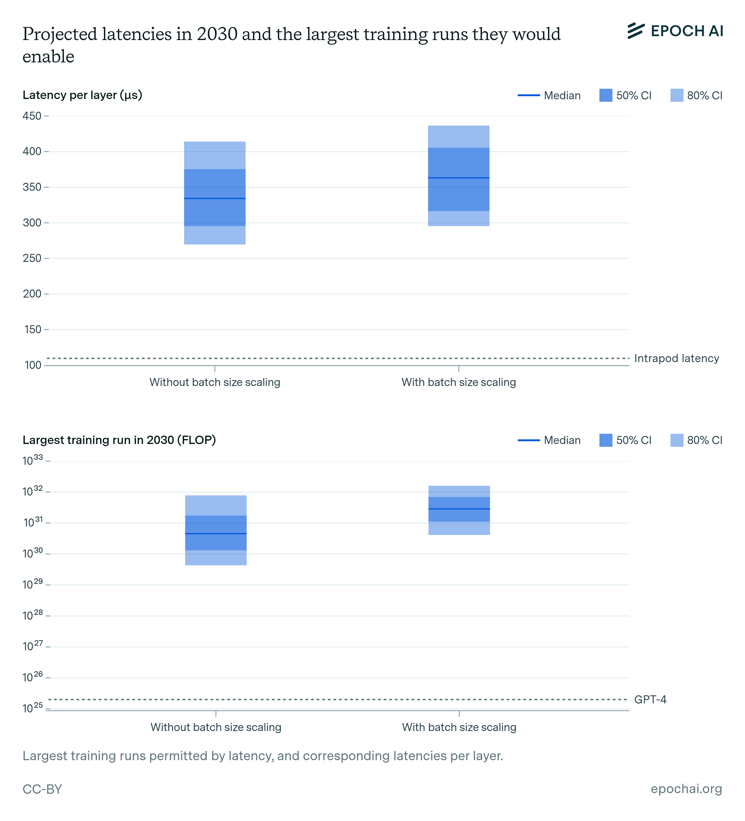
To get a quantitative sense of the size of this bottleneck, we investigate the relevant sources of latency in the context of training large transformer models. Given batch sizes of 60 million tokens (speculated to be the batch size of GPT-4), we arrive at training runs between 2e30 to 2e32 FLOP, which would incur at least 270 to 400 microseconds (µs) of NVLINK and Infiniband communication latency per layer.
However, this may be an underestimate because we expect that the critical batch size likely scales with model size. Under a speculative assumption that batch size can be scaled as roughly the cube root of model size, we estimate the feasibility of training runs around 3e30 to 1e32 FLOP, which would incur at least 290 to 440 µs of latency with modern hardware.92
Latency wall given intranode latencies
We first focus our analysis on intranode latencies, meaning latencies associated with a single node (i.e. a server) hosting multiple GPUs. In this case there are two types of latency that are most pertinent: the kernel latency captures how long a single matrix multiplication or “matmul” takes, and the communication latency measures how long it takes to propagate results between the GPUs.
We anchor our estimates of these two latencies to commonly used machine learning hardware. Experiments by Erdil and Schneider-Joseph (forthcoming) indicate a kernel latency on the order of 4.5 µs for an A100 GPU. Meanwhile, the communication latency in an 8-GPU NVLINK pod for an all-reduce is on the order of 9.2 µs.93 The total base latency per matmul in an NVLINK pod is then in the order of 13.7 µs.
The latency of each transformer layer follows straightforwardly from this. In particular, each layer of a standard decoder-only transformer model involves four consecutive matrix multiplications,94 and we must pass each layer twice (for the forward and backward passes). Therefore, the minimal latency per layer and batch is eight times that of a single matrix multiplication, i.e. \( 8 \times 13.7\,\mu\text{s} = 110\,\mu\text{s} \).
To finish estimating the largest training run allowed by the latency wall, we need to make some assumption on scaling the number of layers and the amount of training data. As a heuristic, let’s assume that the number of layers in a model is roughly the cube root of the number of parameters,95 and that the training dataset size will scale proportionally with the number of parameters, following the Chinchilla rule. In particular, assuming a 120 µs minimum latency per layer and a batch size of 60M tokens, we would find that the largest model that can be trained in nine months is 700T parameters, which allows for Chinchilla-optimal models of up to 6e31 FLOP. Note that this estimate might prove to be too optimistic if the latencies per all-reduce from the NVIDIA Collective Communications Library (NCCL) prove to be slower than reported for intermediate size messages.96,97,98
Latency wall given latencies between nodes
So far we have only accounted for intranode (within-node) latencies. This makes sense to some extent; tensor parallelism is often entirely conducted within 8-GPU NVLINK pods precisely to avoid communicating between nodes for each sequential matrix multiplication. However, continued scaling would require internode communication, increasing the latency.
In particular, using a standard InfiniBand tree topology, the latency between nodes scales logarithmically with the number of nodes communicating. Using the NVIDIA Collective Communications Library (NCCL), an all-reduce operation will take at least \( t = 7.4\,\mu\text{s} + 2 \times \left(N \times 0.6\,\mu\text{s} + \log_2(M) \times 5\,\mu\text{s}\right) \) , where \( N \) is the number of GPUs within a pod participating, and \( M \) is the number of pods participating (this includes both the communication and kernel latencies).99
For a training run using 2D tensor parallelism, the number of pods corresponds be the number of GPUs coordinating for a 2D tensor parallel calculation. In particular, a cluster performing TP-way 2D tensor parallel training requires a synchronization of TP GPUs, for which we will have 2.75 GPUs on average communicating within each 8-GPU pod, and \( \sqrt {\text{TP}} / 2.75 \) pods total.
For instance, a 300M H100 cluster using 2,000-way 2D tensor parallelism would involve then \( \sqrt {2000} / 2.75 = 16 \) pods per all-reduce, incurring a 7.4 µs + 2 x (2.75 x 0.6 µs + log2(16) x 5 µs) = 50 µs latency, which corresponds as before to a 8 x 50 µs = 400 µs latency per layer and batch. This is the cluster size that would allow training the largest possible model in under nine months and with 60M batch size, reaching 7e30 FLOP given projections of hardware efficiency.100
How can these latencies be reduced?
Communication latency might be significantly reduced with improvements to the cluster topology. For instance, a mesh topology could bypass the logarithmic scaling of the internode latency, at the cost of a more complex networking setup within data centers (since you would need to have direct connections between all nodes).
Another solution might involve larger servers with more GPUs per pod, to reduce the internode latency, or more efficient communication protocols—for instance, for training Llama 3.1 Meta created a fork of the NVIDIA Collective Communications Library (NCCL) called NCCLX that is optimized for high latency setups, which they claim can shave off tens of microseconds during communications.
Alternatively, we might look into ways to increase the batch size or reduce the number of layers. Previous research by OpenAI relates the critical batch size – after which you see large diminishing returns to training – to how dispersed are gradients with respect to one’s training data. Based on this, Erdil and Schneider-Joseph (forthcoming) conjecture that the batch size might be scaled with the inverse of the reducible model loss, which per Chinchilla scales as roughly the cube root of the number of model parameters.101 If this holds, it would push back the latency wall by an order of magnitude of scaling, see figure 7 below.
Little work has been done on how the number of layers ought to be scaled and whether it could be reduced. Some experimental work indicates that it is possible to prune up to half of the intermediate layers of already trained transformers with a small degradation of performance. This indicates that removing some layers before training might be possible, though it is far from clear. For the time being, we ignore this possibility.
After accounting for uncertainties, we conclude that scaling past 1e32 FLOP will require changes to the network topology, or alternative solutions to scale batch sizes faster or layers slower than theoretical arguments would suggest.
What constraint is the most limiting?
So far we have examined four main bottlenecks to AI scaling in isolation. When considered together, they imply that training runs of up to 2e29 FLOP would be feasible by the end of the decade. This would represent a roughly 10,000-fold scale-up relative to current models, and it would mean that the historical trend of scaling could continue uninterrupted until 2030 (see figure 7).102
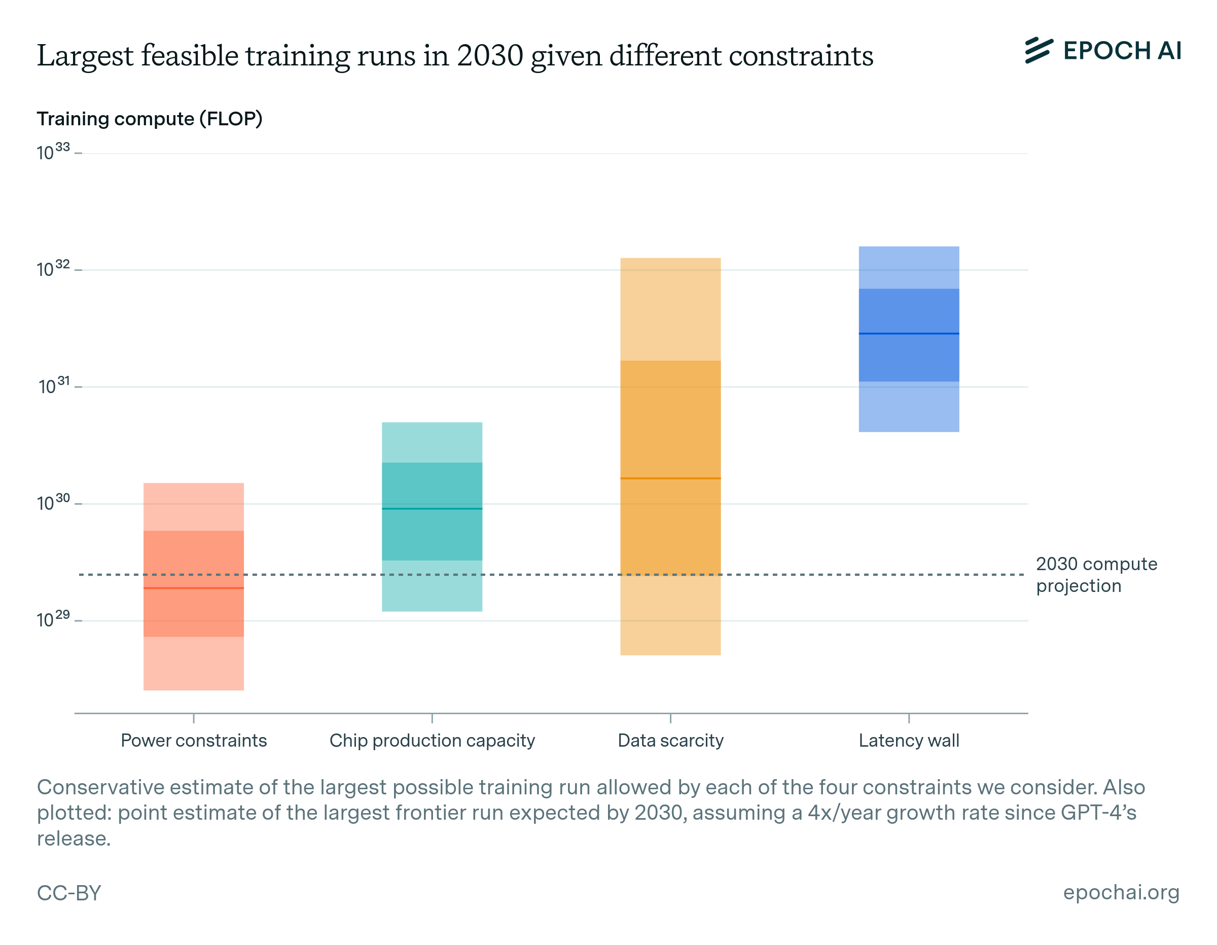
The dark shaded box corresponds to an interquartile range and light shaded region to an 80% confidence interval.
The most binding constraints are power and chip availability—see figure 7. Of these two, power may be more malleable—the energy industry is less concentrated and there is precedent for 100 GW expansion of the power supply, which suppliers ought to be able to execute if planning three to five years in advance. Expanding chip manufacturing faces multiple challenges: key processes like advanced packaging are mostly allocated to data center GPUs already, and building new fabs requires large capital investments and highly specialized labor.
Data stands out as the most uncertain bottleneck, with its uncertainty range spanning four orders of magnitude. The utility of multimodal data for advancing reasoning capabilities may be limited, and our estimates of both the available stock of such data, its quality, and the efficiency of current tokenization methods are less certain than those for text-based data. Ultimately, synthetic data might enable scaling indefinitely, but at a large compute cost.
Lastly, while the latency wall is a distant constraint, it looms on the horizon as an obstacle to be navigated. It might be pushed back by adopting more complex network topologies, involving larger pods or more connections between pods.
Will labs attempt to scale to these new heights?
We find that, based on extrapolating current trends around the key AI bottlenecks, training runs of up to 2e29 FLOP will be possible by the end of this decade. Achieving this scale would be on-trend: The largest training runs to date have been of the order of 5e25 FLOP, and six more years of the historical trend of 4x/year would result in models trained using roughly 2e29 FLOP. The price tag of the cluster needed for such a training run will be on the order of hundreds of billions of dollars.103 Will the AI industry actually seek to train models of this scale?
To date, increasing the scale of AI models has consistently led to improved capabilities. This has instilled a scaling-focused view of AI development that has resulted in the amount of spending on training runs growing by around 2.5x/year. Early indications suggest that this is likely to continue. Notably, it has been reported that Microsoft and OpenAI are working on plans for a data center project known as “Stargate” that could cost as much as $100 billion, set to launch in 2028. This suggests that major tech companies are indeed preparing to achieve the immense scales we’re considering.
Further evidence of AI systems’ potential for sufficiently large economic returns could emerge from scaling beyond GPT-4 to a GPT-6 equivalent model, coupled with substantial algorithmic improvements and post-training improvements. This evidence might manifest as newer models like GPT-5 generating over $20 billion in revenue within their first year of release; significant advancements in AI functionality, allowing models to seamlessly integrate into existing workflows, manipulate browser windows or virtual machines, and operate independently in the background. We expect that such developments could convince AI labs and their backers of these systems’ immense potential value.
The potential payoff for AI that can automate a substantial portion of economic tasks is enormous. It’s plausible that an economy would invest trillions of dollars in building up its stock of compute-related capital, including data centers, semiconductor fabrication plants, and lithography machines. To understand the scale of this potential investment, consider that global labor compensation is approximately $60T per year. Even without factoring in accelerated economic growth from AI automation, if it becomes feasible to develop AI capable of effectively substituting for human labor, investing trillions of dollars to capture even a fraction of this $60T flow would be economically justified.
Standard economic models predict that if AI automation reaches a point where it replaces most or all human labor, economic growth could accelerate by tenfold or more. Over just a few decades, this accelerated growth could increase economic output by several orders of magnitude. Given this potential, achieving complete or near-complete automation earlier could be worth a substantial portion of global output. Recognizing this immense value, investors may redirect significant portions of their capital from traditional sectors into AI development and its essential infrastructure (energy production and distribution, semiconductor fabrication plants, data centers). This potential for unprecedented economic growth could drive trillions of dollars in investment in AI development.104
Settling the question of whether companies or governments will be ready to invest upwards of tens of billions of dollars in large scale training runs is ultimately outside the scope of this article. But we think it is at least plausible, which is why we’ve undertaken this analysis.
Conclusion
In this article, we estimated the maximum feasible scale of AI training runs by 2030 by analyzing the availability and potential constraints key factors required for scaling up training runs. We examined four categories of bottlenecks (power constraints, chip manufacturing capacity, data scarcity, and the latency wall) to determine at what point they might render larger training runs infeasible. Our main result: Based on current trends, training runs of up to 2e29 FLOP will be feasible by the end of this decade. In other words, it is likely feasible, by the end of the decade, for an AI lab to train a model that would exceed GPT-4 in scale to the same degree that GPT-4 eclipses GPT-2 in training compute.
One of the most likely reasons that training runs above these scales might be infeasible is the amount of power that can be supplied by the grid. Substantially expanding the data center power supply by 2030 may be challenging due to grid-level constraints, carbon commitments, and political factors.
The second key constraint is the limited capacity to manufacture tens of millions of H100-equivalent chips per year. Capacity might be limited if capital expenditure is not substantially accelerated through the next decade, even if the relevant manufacturing capacity is mostly dedicated to producing GPUs or other AI accelerators.
Overall, these constraints still permit AI labs to scale at 4x/year through this decade, but these present major challenges that will need to be addressed to continue progress.
If AI training runs of this scale actually occur, it would be of tremendous significance. AI might attract investment over hundreds of billions of dollars, becoming the largest technological project in the history of humankind. Sheer scale translates into more performance and generality, suggesting that we might see advances in AI by the end of the decade as major as what we have experienced since the beginning of the decade.
Finally, through our work we have grappled with the uncertainty we face in predicting the trajectory of AI technologies. Despite their importance, power restrictions and chip manufacturing stand out as uncertain. We will be investigating these in more depth in future work.
We thank Anson Ho, David Owen, Konstantin Pilz, Benjamin Todd, Romeo Dean, Michael Dickens, Max Negele, David Schneider-Joseph, Andy Lubershane, Natalia Martemianova, Ying Yi, Luke Frymire, Peter Wildeford, Jean-Stanislas Denain, Trevor Gaunt, David Mathers, Dylan Patel, Carl Shulman, Ajeya Cotra, Alexander Erben, Ryan Greenblatt, Tim Fist.
Appendices
Appendix A: Summary of the extrapolative model
Our simple extrapolative model of bottlenecks has four components, modeling each of the main bottlenecks we discuss in the article. The code for the model can be found here, and the default model parameters with sources can be found here.
First, for modeling power restrictions we consider the installed power capacity of data centers across the US. This is scaled according to projections of data center demand by local utility providers, and restricted by projections of growth of total US power capacity growth. We also separately model the trend of growth of non-AI data centers, which we constrain to grow only at most as fast as the overall data center capacity growth. The projected capacity for AI data centers is modeled as the difference between the projected total data center capacity and the projected non-AI data center capacity. A fraction of this (modeled following Appendix B) is our final estimate of the available capacity for a single training run. We combine this estimate with an exponentially improving trend of energy efficiency (in FLOP/s/W) and estimates of training run length to compute a largest possible training run. We take the minimum between this and the distribution of training runs sizes allowed by plausible achievable bandwidths, as described in the feasibility of distributed training runs section. We also take the maximum between this result and the largest local training run defined by a distribution over plausible local power supplies by 2030.
Second, for modeling limited chip manufacturing capacity, we consider the current bottlenecks of CoWoS packaging and high-bandwidth memory (HBM) production. We project GPU production to grow between 30% and 100% per year, which aligns with recent scale-ups and expected growth in CoWoS and HBM. The model limits this GPU production trend by a projection of TSMC’s total wafer production for <7nm nodes. However, this limit does not have a significant effect by 2030, based on our chosen parameters. We assume that the compute stock accumulates over time, with new chips improving in FLOP/s by 44% per year. As with the power model, this is combined with estimates of the fraction of the stock available, the training run length, and utilization to estimate a largest possible training run.
Third, the model based on data considers the existing stocks of text, video and image. They are combined according to some estimates of transfer efficiency. Finally, we model them as growing exponentially at a rate congruent to the historical rate of growth of internet content. To convert the effective data stock into a maximum training run size we use Chinchilla scaling of 20 tokens per parameter, and total training compute equal to six times the parameter count times the training dataset size.
Fourth and last, to compute the latency wall limit we solve a system of equations as detailed in appendix E. This considers how the communication latency scales with the number of GPUs that need to synchronize to perform tensor parallelism, while accounting for batch size scaling, layer depth scaling and improvements in hardware performance.
All model parameter choices are informed by evidence we could find and our own guesses and intuitions. Model inputs are assumed to follow a metalog distribution that fits our guesses of the 10%, 50% and 90% distribution percentiles. We further constrain percentage parameters to be withing 0% and 100%, and growth rates to be above 1. We also induce a correlation between the parameter via a Gaussian copula. The correlations induced are explained in table 1 below.
Appendix B: Fraction of total resources allocated to the largest training run
When modeling electrical power and chip manufacturing capacity, we must consider how competition between AI labs affects the fraction of these resources that a lab can secure to perform the largest training run. To estimate this fraction, we consider the stock of AI chips available to each of the most well-resourced firms at the beginning of 2024. We then divide each firm’s stock by the total stock of AI chips available. Finally, we adjust this fraction down to account for some chips being allocated to inference. For convenience, we measure the stock of AI chips in terms of H100-equivalents: the number of Nvidia H100 GPUs that would match the total FLOP/s of the stock, at 16-bit precision. Full calculations are available here.
Meta: According to analyst firm Omdia, Meta acquired 150,000 H100 GPUs by the end of 2023. Meta plans to have a total of 600,000 H100-equivalent GPUs by the end of 2024. So it is likely that Meta’s stock of H100-equivalents at the beginning of 2024 was between 150,000 and 600,000.
Microsoft: Omdia estimates that Microsoft also acquired 150,000 H100 GPUs by the end of 2023. Microsoft reportedly plans to triple their stock of AI chips to 1.8 million by December. It is unclear what kind of chips these will be, but the plan implies that the initial stock was 600,000 chips, and the timing suggests that many of the new chips will be H100s. Based on the rate of hardware efficiency improvements, the initial stock of 600,000 chips would equate to around 300,000 H100 equivalents.105 However, it is unclear exactly when Microsoft’s expansion plans started. Microsoft may have already acquired more H100 GPUs by the start of 2024; we estimate up to 140,000.106 Accounting for all of this, we believe that Microsoft’s stock of H100-equivalents at the beginning of 2024 was likely between 150,000 and 600,000.
Google: Little is known publicly about the production of Google’s custom AI chips, known as TPUs. However, one report by analyst firm TechInsights estimates the total number of TPU shipments each year.107 Based on the release dates of each generation of TPU, it is likely that most of the estimated 2 million units in 2023 and 1.5 million units in 2022 were TPUv5. However, there are two versions of TPUv5: the more efficient TPUv5e, and the higher-performance TPUv5p. The share of each TPU type is unclear, so we estimate the total number of TPUv5 units shipped to be between 1 and 3.5 million, and the share of that total made up by TPUv5p to be between 10% and 90%.
As for TPUv4, which was released in 2021, we believe that peak production likely occurred between 2020 and 2022, and estimate that a total of 250,000 to 1.5 million units were produced based on the yearly production reported by TechInsights. We neglect older generations of TPU, given the much lower estimates of production prior to 2021 and the lower performance of those older generations. Google also owns Nvidia GPUs, but given the track record of Google labs exclusively using TPUs to train their flagship models, we think it is unlikely they will allocate these GPUs to their largest training run. So putting the TPUv4 and TPUv5 numbers together, we estimate that the total number of H100-equivalents available to Google is between 400,000 and 1.4 million.
Amazon: According to the Omdia report, Amazon acquired 50,000 H100 GPUs by the end of 2023, which is three times less than Microsoft and Meta. Amazon also has custom Trainium chips, with one report that Amazon Web Services (AWS) will soon offer clusters of up to 100,000 Trainium2 chips with a peak of 65e18 FLOP/s of compute. This corresponds to about 66,000 H100-equivalents assuming FP16 precision, or 33,000 assuming FP8 precision. If Amazon already has several of these clusters, they may have hundreds of thousands of H100-equivalents in total. Given that these clusters are only just coming online, however, it seems unlikely that Amazon’s stock of AI chips would exceed Google’s estimated stock of 400,000 to 1.4 million H100-equivalents.
Total stock: To estimate the total stock of AI chips available for training by the beginning of 2024, we add up actual H100s shipped, other GPUs, and Google TPUs. The actual H100s shipped was likely between 500,000 and 1.6 million. Omdia estimated a total of 650,000 shipped to major companies. Given Nvidia’s annualized data center revenue of $47.5 billion, and a price of $30,000, they could only have sold about 1.6 million H100s at most.
Other GPUs likely make up between 200,000 and 1 million H100 equivalents. The peak years for the previous generation A100 were 2021 and 2022, in which Nvidia earned a combined $25 billion in data center revenue. At $15,000 per unit, this implies at most 1.7 million units sold, corresponding to about 500,000 H100 equivalents. A more conservative estimate would be $15B / $20,000 ~= 750,000 A100s—roughly 250,000 H100 equivalents. Besides the A100, other GPUs would have a smaller contribution, as they either have lower performance or a much smaller share of the market. Above, we estimated that Microsoft’s 150,000 H100 GPUs imply roughly double that number in total H100 equivalents; a similar argument here implies at most 500,000 * 2 = 1 million H100 equivalents from non-H100 GPUs.
Training allocation: Available computing resources are split between training new models and running inference on existing ones. A simple analysis suggests AI labs should allocate comparable resources to both tasks. Assuming this balance, we can estimate future resource allocation. If in 2029 training and inference compute are equal, and training compute continues to grow at 4x per year, one-quarter of total compute (equal to 2029’s training) will run inference on 2029 models, while three-quarters will train 2030 models. This suggests that 80% of 2030’s compute would be used for training new models, while 20% would be used for inference on previous models.
Result: Adding the stock of actual H100s, other GPUs, and TPUs together results in an estimate of 1.5 to 3.5 million H100-equivalents in total by the beginning of 2024. Since Google has the highest stock estimate of 400,000 to 1.4 million H100-equivalents, we use this stock to estimate the allocation of total resources. After adjusting for 80% of a company’s compute being spent on training, our final result is that the largest training run can be allocated 26% (somewhere between 16% to 40%) of the total available chip stock.
Appendix C: Bandwidth constraints
Suppose we have a ring all-reduce setup involving \( M \) data centers, with fiber optic bandwidth \( F \) bps between every data pair and \( t_L \) seconds of latency for a round trip across the network.
The standard all-ring reduce includes \( M-1 \) stages of parallel reduce followed by \( M-1 \) stages of broadcast. In each stage, peers communicate to their next neighbor a tensor of size \( N/M \), where \( N \) is the size of the model, which can be communicated in \( N/M \times 8 / F \) seconds, assuming 8 bits per parameter. In total, this takes \( 2(M-1) \times N/M \times 8 / F \approx 2 \times N \times 8 / F \) seconds.
To this we need to add the latency, corresponding to two round trips down the network, for a total time per all reduce of:
\[ t_{\text{AR}} = \frac{2 \times N \times 8}{F} + 2 \times t_L \]
Following a logic similar to what is explained in the section Feasibility of distributed training runs when talking about latencies, this would lead to a maximum of \( U = \frac{T}{t_{\text{AR}}} \) gradient updates, allowing for a dataset size of \( D = U \times B \) , where \( B \) is the maximum achievable batch size.
We assume the usual Chinchilla relation between model size and number of parameters (\( D = 20 \times N \)), and numerically solve for the largest model that can be trained using the fsolve facility in scipy.
Appendix D: Equivalence between multimodal and text data
Here we set out to estimate how many tokens an image or second of video would be encoded as, in relation to one token of text.
Establishing an equivalence rate between data of different modalities is complex. In the limit, we expect multimodal tokenizers to encode media with an amount of tokens roughly proportional to the amount of information therein contained. So we try to estimate how much information image and video data have in relation to text.
Henighan et al (2020) estimate that one 32x32 image provides an information gain over a description as the equivalent of 2-3 words (eg 2-4 tokens of text), which we take as a lower bound on the information content of an image. Chameleon-34B encode 512x512 images using 1024 text-equivalent tokens, i.e. 770 words. As of June 2024, OpenAI charges 255 text tokens to process 512x512 images with GPT-4o. Yu et al (2023) encode images with good performance using 256 tokens with a dictionary of 218 tokens, four times bigger than typical text tokenizers; we take that as equivalent to \( 256 \times 18/16 \approx 290 \) text tokens (typical text tokenizers use a codebook with 216 entries, hence the adjustment). Yu et al (2024) encodes 256x256 images using 32 tokens from a codebook with 211 entries, equivalent to \( 32 \times \frac{11}{16} = 22 \) text tokens. While the Chameleon paper is the most straightforward application, given the rest of the evidence pointing towards lower dimensions we consider a range of 2 to 290 tokens per image.
For video, we speculate that one second of video content would be the equivalent of 2-10 words of content based on typical speech speeds, i.e. 2-13 text tokens. The information in a video is highly redundant compared to images—for instance, typical high res images take up 2MB of space, while 720p/1080p videos take up 1GB of space per hour of video, ie 0.2MB per second of video, which would suggest there is less information per second of video than in ten images. So we take as lower bound the 2 tokens per second of speech and as an upper bound the same 290 tokens per second that we assigned to an image, as a generous upper bound of the image content in the video.
Thus we arrive at a rate of 2 to 290 tokens per image or second of video. We consider this an extremely rough guess, and acknowledge there is significant room for disagreement.
Appendix E: Computing the largest possible training run given variable communication latency restrictions
In this appendix we explain how we estimate the largest model that can be trained using a tree topology setup without running into latency constraints.
The latency per layer and batch \( t_L \) corresponds to combining the base comms latency \( t_{\text{base}} \) and the variable comms latencies within a node \( t_{\text{INTRA}} \) and across nodes \( t_{\text{INTER}} \). Here we are assuming 8-GPU NVLINK nodes (of which at most \( \lceil \sqrt 8 \rceil = 3 \) coordinate after each layer), and a tree structure, using the formula for an all-reduce latency found in the NCCL repository. We multiply this by 4 since each layer has an attention and MLP block, which need to be traversed forward and backward for each batch during training.
\[ t_L = 4 \times \left[t_{\text{base}} + 2 \times \left(t_{\text{INTRA}} \times 3 + t_{\text{INTER}} \times \max\left(0, \log_2\left(\frac{\text{TP}_\text{RANK-2D}}{8}\right)\right)\right)\right] \]
The number of ranks involved in 2D tensor parallelism synchronization after each layer (\( \text{TP}\_\text{RANK-2D} \)) is the square root of the number of ranks involved in tensor parallelism overall. We bound this as inversely proportional to the maximum slicing across GPUs that can be achieved with data and pipeline parallelism, considering the minimum number of samples in a batch \( B_{\text{MIN}} \) that can be processed with TP efficiently (\( DP_\text{RANK} \times PP_\text{RANK} = \frac{B}{ B_{\text{MIN}}} \)).
\[ \text{TP}_\text{RANK-2D} = \max\left(1, \sqrt{\frac{n_{\text{gpu}} \cdot B_{\text{MIN}}}{B}}\right) \]
To estimate \( B_{\text{MIN}} \) in the first place we need to look into the utilization that GPUs can achieve given their bandwidth. This utilization is optimized when the amount of time spent on memory accesses is roughly equal to the time spent on computation. For language transformers, we will be multiplying tensors with dimensions \( (B_{\text{MIN}}, d_{\text{ff}}, d_{\text{model}}) \), which roughly require \( B_{\text{MIN}} \times d_{\text{model}} \times d_{\text{ff}} \) multiply-adds and \( B_{\text{MIN}} \cdot d_{\text{model}} + d_{\text{model}} \cdot d_{\text{ff}} + B_{\text{MIN}} \cdot d_{\text{ff}} \) read-writes, where dff and dmodel are the feed-forward and model dimensions respectively. Assuming a peak hardware performance of H FLOP/s, a bandwidth of W bytes/s and a parameter precision of p bytes, the equilibrium between memory access and computation will be achieved when:
\[ \frac{2 \text{FLOP/multiply-add} \times \# \text{multiply-adds}}{H} = \frac{\# \text{read-writes} \times p}{W} \]
\[ \frac{2 \times B_{\text{MIN}} \times d_{\text{model}} \times d_{\text{ff}}}{H} = \frac{(B_{\text{MIN}} \times d_{\text{model}} + d_{\text{model}} \times d_{\text{ff}} + B_{\text{MIN}} \times d_{\text{ff}}) \times p}{W} \]
\[ \frac{2 \times W}{H \times p} = \frac{1}{B_{\text{MIN}}} + \frac{1}{d_{\text{model}}} + \frac{1}{d_{\text{ff}}} \]
For a sufficiently large model, the right side of this equation simplifies to \( 1 / B_{\text{MIN}} \), and we have that:
\[ B_{\text{MIN}} = \frac{H x p}{2 x W} \]
For the H100 at FP8 precision, the minimum batch size per GPU would then correspond to \( B_{\text{MIN}} = \frac{2e15 \text{ FLOP/s} \times 1 \text{ byte/param}}{2 text{ FLOP/multiply-add} \times 3e12 \text{ bytes/s}} \approx 330 \). Theoretically, this minimum batch size would increase over time, as the bandwidth and hardware performance improve unequally fast. For simplicity of the analysis, we assume that it will stay roughly fixed.
The number of GPUs is approximated by the model compute \( C \) divided by the training duration \( T \) and the utilization-adjusted hardware performance \( H \) (this is an underestimate, as utilization worsens with scale).
\[N_{\text{GPU}} = C(T \times H)\]
The model compute \( C \), dataset size \( D \) and model size \( N \) obey the usual relation.
\[C = 6DN\]
And dataset size \( D \) is assumed to scale in relation to model size \( N \) following the Chinchilla rule.
\[D = 20 \times N\]
The batch size \( B \) and the layer depth \( L \) are assumed to grow exponentially with respect to model size (if assuming that batch size doesn’t scale then just take \( B \) as given).
\[B = B_0 \times N^\alpha_B\]
\[L = L_0 \times N^\alpha_L\]
The minimum training time \( T \) is then bounded by time per layer and batch size \( t_L \) times the number of layers \( L \) times the number of gradient updates (\( U = D/B \)). In the point where scale is maximized, this limit will be taut.
\[T = t_L \times L \times D/B\]
We solve this system of equations numerically using the fsolve facility in scipy.
Appendix F: Unprecedented economic growth could drive massive AI investment
In the section “Will labs attempt to scale to these new heights?”, we argued that the unprecedented economic growth from AI automation could drive massive AI investments. While this is far from guaranteed, in this appendix we outline a rough calculation to illustrate this dynamic.
The starting point is to consider a lifetime value function \( V \), with isoelastic flow utility over consumption \( c \). To capture the economic impact of massive AI automation, we assume that consumption is constant at \( \bar{c} \) until some year \( T \), after which consumption goes to infinity. We then have
\[V(c,T) = -\sum_{t=0}^T \beta^t \bar{c}^{-\gamma} = -\bar{c}^{-\gamma} \frac{1-\beta^{T+1}}{1-\beta},\]
where we sum over years \( t \) with discount \( \beta \) and elasticity of intertemporal substitution \( \gamma \).
The next step is to relate this to AI investment – in particular, we consider how much flow consumption a representative agent would be willing to bring forward the arrival date of these economic impacts. Let’s say the representative agent is indifferent between a consumption of \( c_1 \) in year \( T_1 \) and a consumption of \( c_2 \) in year \( T_2 \), i.e. \(V(c\_1, T\_1) = V(c\_2, T\_2)\). Then it follows that
\[ \frac{c_1}{c_2} = \left(\frac{1-\beta^{T_1+1}}{1-\beta^{T_2+1}}\right)^{\frac{1}{\gamma}}\]
With this expression, we can now plug in some plausible numbers for illustration. Suppose we want to move the point of massive automation from \( T_2 = 30 \) years to \( T_1 = 20 \) years, with a discount rate of 2% (i.e. \( \beta = 0.98 \)) and \( \gamma = 1 \) (Havránek et al. 2015). Then we have \( \frac{c_1}{c_2} \approx 0.74 \), implying that it is worth giving up 26% of flow consumption each year!
In the US, around 70-80% of GDP is dedicated to consumption (World Bank, 2022), amounting to around $18.75T each year. If we believe the above calculation, this suggests forfeiting around $4.7T worth of consumption annually to hasten the arrival of massive automation. Of course, this calculation is based on aggressive assumptions, but at the very least it illustrates why massive upfront investments in AI infrastructure might make sense.
Notes
-
For LLMs, compute scaling likely accounts for the majority of pre-training performance gains. Post-training techniques can add substantial but highly variable improvements, depending on the specific method and domain. When considering both, the relative importance of compute scaling becomes less clear. ↩
-
GPT-2 was trained on around 2e21 FLOP, and GPT-4 was trained on around 2e25 FLOP, a 10,000x increase. ↩
-
Note that the estimate for the largest training run given latency constraints might be too optimistic, since we suspect the communication latencies for the multiplication of intermediate size matrices might be less efficient than we estimate. ↩
-
In this summary and throughout this article, whenever a range is given it is to be understood as an 80% CI. ↩
-
However, note that other countries might end up being preferred by developers. For example, Chinese providers installed over a terawatt of power in the last decade, and the UAE has a friendly regulatory process for securing power. ↩
-
We are assuming training runs between 2 and 9 months of duration, and that for distributed training a single company will only be able to leverage between 16% and 40% of the available supply of power for AI data centers. ↩
-
That is, the state-of-the-art among GPUs that are currently widely used. Nvidia has already announced its next generation of Blackwell chips. We account for future GPU generations by projecting efficiency improvements through 2030. Note that Google DeepMind mostly uses Google TPUs for training, but we use Nvidia as our baseline because there is more available information on NVIDIA products than TPUs, and because they are overwhelmingly popular among the AI industry overall. ↩
-
Based on the average ratio between the H100 DGX SuperPOD server expected average power (EAP) to the TDP of individual GPUs, we find an overhead factor of 1.4MW / 1016 GPUs / 700W per GPU = 1.96x (see Table 4 here). Additionally, the power usage effectiveness (PUE), which accounts for data center-level overhead like cooling and power distribution, in e.g. Patterson et al (2021) is reported as a 1.2x additional factor. This results in 700 * 1.96 * 1.2 = ~1700W per GPU. Here we follow our previous work (see Appendix A.4 from the paper). ↩
-
The average US household consumes 10,000 kWh of electricity a year, for an average rate of ~1,200 W after dividing by 8,760 hours in a year. ↩
-
Training compute for frontier models is growing as 4.1x/year, which would result in training runs of \( 3.8e25 \text{ FLOP} \times 4.1\text{ x/year}^{6\text{ years}} = 2e29\text{ FLOP} \) by end of the decade. ↩
-
We derive this from an expansion of our previous research on the ML hardware power-efficiency trend. ↩
-
4-bit training has been discussed and demonstrated in particular research contexts, but it isn’t clear whether it will be useful in practice. We conservatively assume it won’t be. ↩
-
It’s not possible to use the full capacity of 1200 GW capacity in practice, because sources like solar, wind, and hydroelectricity generate power intermittently. In addition, power demand naturally fluctuates over time. The US generated over 4,178 terawatt-hours in 2023; 4178 TWh / 8760 hours in a year = 477 GW of power generation on average. ↩
-
See the section “Power constraints for geographically distributed training” for more discussion on this figure. ↩
-
One interesting case study is pump storage facilities. Bath County in Virginia houses the largest pumped storage station in the US, with an potential output capacity of 3GW. The input capacity is likely similar—”When generating power, the water flow can be as much as 13.5 million US gallons (51,000 m3) per minute (850 m3/s). When storing power, the flow can be as much as 12.7 million US gallons (48,000 m3) per minute (800 m3/s).” Another point of comparison is CERN’s Large Hadron Collider, which peaks at 200 MW consumption. ↩
-
Note that since solar farms output varies with the time of the day, the average capacity is roughly 4x less than nominal capacity. ↩
-
Notably, all of them are either hydroelectric, nuclear or based on fossil fuels. ↩
-
Major electricity consumers secure power through long-term contracts, so power from large plants will be at least partly locked by contracts. In addition, one expert we consulted stated that the US has little spare power capacity given existing supply, since many parts of the US are at “elevated risk” of power shortfalls. ↩
-
We could find just two US plants with capacity over 3GW constructed after the year 2000: the Manatee oil plant and the West County Energy Center in Florida. Most other power plants over 3GW were constructed in the 1970s. The West County Energy Center construction permit was conceded in March 2006 and finished construction of its third reactor by July 2011, suggesting that it is feasible to build >3GW power plants in five years. ↩
-
We emphasize that this applies to power stations already existing or planned. A determined actor might be able to build their own large scale power stations over 3 GW. ↩
-
The largest utility company in Northern Virginia (Dominion) has connected over 4 GW of data centers since 2019, and has 5.8 GW of contracts with data centers. NOVEC, another Northern Virginia utility, also serves many data centers, but is a much smaller utility overall at 175k customers versus Dominion’s 2.7 million. ↩
-
Dominion projects an annual growth rate of 10%, which would be an ~1.8x increase over six years. See the next section for more details on growth projections. Note that providers are likely to update their plans for expansion as the demand for such large data centers becomes clearer—and there is precedent for aggressive expansion when facing unexpected demand. For instance, in 2022 Georgia Power said “it will need 17 times more electricity—the equivalent of four new nuclear units—than it had forecast just 18 months earlier because of new data centers and manufacturing in the state.” ↩
-
“The executives [at Microsoft and OpenAI] have discussed launching Stargate as soon as 2028 and expanding it through 2030, possibly needing as much as 5 gigawatts of power by the end”, Stargate being the codename for the proposed project. ↩
-
We assume a 4x increase in FLOP/s per W over the H100s, and FP8 performance. 100 days, which is similar to today’s training runs, would result in ~7e28 FLOP. ↩
-
Gemini technical report: “Training Gemini Ultra used a large fleet of TPUv4 accelerators owned by Google across multiple data centers”. It is not clear how many data centers were split across, or if they were close by. ↩
-
See their ISO 27001 compliance report for the locations. ↩
-
Currently, data centers in the US likely consume over 20 GW of power, on average: The IEA estimates that US data centers consumed “around 200 TWh in 2022 (~4% of US electricity demand)”, which would be an average rate of ~23 GW over the year. Meanwhile, McKinsey estimates US data centers consumed 17 GW on average in 2022, and Goldman Sachs estimates 146 TWh in 2023, or ~17 GW on average. Given this range of estimates, and rapid growth in recent years, the current rate is likely above 20 GW. ↩
-
20 / 0.6 = 33.3, and 20 / 0.4 = 50. ↩
-
SemiAnalyis reports the critical IT capacity (see Figure 2) without accounting for power usage effectiveness (PUE), which is total data center power divided by power used directly for compute rather than overhead functions such as cooling. Our estimate of power consumption per GPU also includes this overhead, so we need to use the total capacity, not the IT capacity. We arrive at our estimates of 36 GW and 48 GW by assuming a PUE of 1.5x for non-AI data centers, and a PUE of 1.2x for AI data centers, based on SemiAnalysis estimates. ↩
-
This is based on backing out growth rates from two different projections. First, Dominion projects that data center capacity will double from 2023 to 2028. 2x growth over 5 years is ~15% annual growth. Another projection from a grid operator is that Dominion’s data center load will grow by 4x over 15 years, and 4^(1/15) = ~1.1, or 10% growth. The shorter-term projection is likely more relevant since we are discussing growth until 2030. ↩
-
From the figure above we can read 22,109 MW and 2,537 MW of installed IT capacity for non-AI and AI datacenters, respectively. Assuming a PUE of 1.5x for the former and 1.2x for the latter, AI datacenters correspond to \( 2{,}537\,\text{MW} \times 1.2\,\text{PUE} \approx 3\,\text{GW} \) installed capacity, which is equal to \( \frac{3\,\text{GW}}{22{,}109\,\text{MW} \times 1.5\,\text{PUE} + 3\,\text{GW}} \approx 8\% \) of total installed capacity. ↩
-
Goldman Sachs projects an increase in non-AI data center energy use from 165 TWh in 2024 to 304 TWh in 2030, which would be a 10.7% growth rate. SemiAnalysis estimates a 8% growth rate in non-AI critical IT capacity between end of 2023 and end of 2028. Recent annual growth in non-AI IT capacity in North America according to SemiAnalysis data was between 11% to 13%. ↩
-
For comparison, both Goldman Sachs and SemiAnalysis expect a planned expansion of AI power demand of more than 2x throughout 2024. This is from a small base, so it’s unclear how long it can be kept up. ↩
-
This is based on each company’s current share of the total stock of AI chips available, measured in units equivalent to the Nvidia H100 GPU. We based the share of power capacity on the share of chips because there was more relevant data available, and there is a strong correlation between power capacity and the number of chips. Our best guess is that Google currently has the largest share, at 33% (20% to 50%). See Appendix B for further details. It’s possible that some companies might choose to reserve a substantial fraction of their resources for inference; here we implicitly assume they will dedicate a majority of their resources to a training cluster, which later might be reused for inference. ↩
-
Gemini technical report: “Training Gemini Ultra used a large fleet of TPUv4 accelerators owned by Google across multiple data centers”. ↩
-
This corresponds to a 11,000km ring network connecting all major data center hubs in the US. We assume that the signal propagates at 200,000 km/s. This is a pessimistic assumption—distributed data centers need not be spread this far apart. We also consider the latency of switches for sending packets. Modern ethernet switches like Marvell’s Teralynx 10 have latencies in the order of 500 ns per packet forward, which can be ignored in comparison to the much larger flight latencies. ↩
-
Under chinchilla-optimal scaling, a model should be trained on 20 tokens per parameter. And training a model requires 6 FLOP per token and per parameter. So the FLOP would be 6 x 1.4e16 x 1.4e16 / 20 = 5.88e31. ↩
-
Other fiber optic solutions such as Infinera’s GX series might achieve better performance, boasting 1.2 Tbps per fiber and wavelength. ↩
-
The math is slightly complex, as more bandwidth results in us being able to train larger models, but larger models take longer to perform gradient updates. We explain the calculation in Appendix C. ↩
-
Note that the switch-router paradigm might not be how data centers coordinate. For instance, multiple nearby data center can be connected via protocols like RDMA over Converged Ethernet (RoCE) to coordinate large training runs without routers mediating the connection. Still, we consider the B4 network an illustrative example of the bandwidth that hypercalers can achieve between larger data centers. ↩
-
We derive this interval from a bootstrapped exponential regression involving 33 ASIC switch controllers announced between 2001 and 2023. ↩
-
Increasing fiber capacity would require increasing the number of ports or the bandwidth per fiber. While long range connections up to 700Tbps per fiber have been demonstrated, experts we consulted believe that in commercial settings we should expect bandwidths per fiber up to 3 Tbps, as techniques applied in research setting to go beyond these connections rely on technologies like Spatial Domain Multiplexing that are believed to be commercially inferior to increasing the number of fibers. The historical trend would suggest 600 Tbps / 128 ports = 5 Tbps by the end of the decade, which is roughly congruent with the expert assessment, suggesting that the trend can in fact be continued up to this point. ↩
-
Two relevant cost examples for bandwidth expansion: the 200 Tbps, 6,000km MAREA trans-atlantic cable cost $165 million, while commercial 200G last-mile underground fiber deployment ranges from $11.30 to $24.13 per foot. These costs might not be very representative of land inter datacenter connections. ↩
-
This estimate corresponds to the distributional minimum of the training runs allowed by distributed power and bandwidth. ↩
-
This last estimate corresponds to the distribution maximum of the previous estimate and the training runs feasible in a single data center campus. ↩
-
One natural question is whether AI developers could simply outbid existing users to acquire more power, independent of supply growth. In the US, utilities are heavily regulated and are overseen by commissions that scrutinize their pricing decisions. This could limit how much data centers can outbid others for power. ↩
-
Full development time, including planning, permitting, and construction, would take longer. Solar plants require <2 years including planning time but not including permitting. ↩
-
Globally, nuclear plants average 6-8 years, but the most recent nuclear plant in the US, Vogtle, took ~14 years. Major hydro plants such as Bath County and Grand Coulee appear to have required roughly 10 years. Wind power timelines seem quite variable and it is unclear what the distribution is. ↩
-
Though a few recently-closed nuclear plants may be reopened within a shorter time frame. There are also companies working on various types of next-generation nuclear plants, including two companies backed by Sam Altman, but these seem unlikely to be deployed at scale by 2030. ↩
-
Solar power is arguably cheaper than gas overall, but requires higher upfront capital costs in exchange for very low operation costs: the EIA estimates that solar power with batteries has a capital cost of over $2k/kW; adjusting for solar’s intermittency, this would be greater than $8k/kW. Companies seeking to scale up power very aggressively may have high discount rates and prefer gas for that reason. ↩
-
A 2020 paper estimates that carbon capture would add 3.87 cents per kWh to the cost of gas. Another estimate is that carbon capture for gas costs $79 to $88 per tonne of CO2 emissions. Given that natural gas produces ~1 pound, or ~1/2000 tonnes of CO2 per kWh, this also implies ~4 cents per kWh. ↩
-
1700 W over 270 days is ~11,000 kWh, or ~$1800 at 17 cents per kWh. ↩
-
However, the total capacity of projects in the interconnection queue is enormous at 1480 GW, so it is not clear how binding this constraint is. Most projects that apply for interconnection are ultimately withdrawn, so this does not imply that 1480 GW of capacity will come online in the coming years. ↩
-
There is bipartisan interest in making it easier to approve new power plants and energy infrastructure. ↩
-
There isn’t a consensus on whether clean energy or fossil fuels are most apt for powering AI growth. NextEra’s CEO said that wind and solar are more promising than gas, while Ernest Moniz, former US secretary of energy, believes that data centers will have to rely heavily on fossil fuels. In any case, constraining the set of possible energy sources presumably would make a scale-up more difficult. ↩
-
Some coal plant retirements have already been delayed due to data center demand. ↩
-
Throughout this section, we focus on Nvidia due to its dominant market share. However, we expect that AI chips from other firms, including Google TPUs, will face similar constraints to scaling production. The AI chip supply chain is highly concentrated in foundries like TSMC, SK Hynix, and Samsung, so different chipmakers will face similar constraints. ↩
-
Assuming that one lab amasses ~1/4th of the 2 million H100s for training (see Appendix B), with 2e15 FLOP/s at FP8 precision, 40% FLOP/s utilization, and 6 months of training. ↩
-
16 million GPUs performing 2e15 FLOP/s each at 40% utilization over 6 months can perform 2e29 FLOP. ↩
-
This is even after assuming that performance improvements continue improving at historical rates of around 40% per year, which would be sufficient for an 8-fold increase in performance, not enough for a 20x increase in total FLOP. ↩
-
A wafer is a large piece of silicon that is used to produce many dies, which are packaged into chips. One wafer can produce enough dies for 28 H100 chips. ↩
-
It is unclear when full capacity will be reached. ↩
-
This does not mean that the number of chips itself will grow at this rate, especially if, as with the Nvidia B200, multiple dies will be packaged into a single chip. ↩
-
Sustaining the trends in AI chip performance may require a new packaging paradigm other than CoWoS in the future, which may require transitioning to new production lines. While this adds some uncertainty, our model assumes that future growth will be similar to the recent and planned levels of growth in CoWoS. ↩
-
We estimated an average of about 50,000 3nm wafers and 130,000 5nm wafers per month for Q4 2023, based on corresponding revenue reports and estimated wafer prices. Similarly, China Times reported that 60k to 70k 3nm wpm was expected by the end of 2023. Combining the 5nm and 3nm figures, the total monthly production for 5nm and 3nm process nodes at the start of 2024 was likely to be around 180,000. This translates to an annualized production volume of 2.2M wafers using these advanced process technologies. Note that NVIDIA H100 GPUs are manufactured on a specialized TSMC 4N node, but this node is included under 5nm in TSMC’s revenue reports. ↩
-
Assuming 28 H100 dies per wafer after accounting for defects, 2 million H100 GPUs would require about 71,429 wafers. Using the estimate of 130,000 5nm wafers per month for early 2024, this represents roughly 5% of TSMC’s annualized 5nm wafer capacity (71,429 / (130,000 * 12) ≈ 4.6%). ↩
-
This can be approximated as \( revenue_{growth} - \frac{margin_{growth}}{100} \), where \(margin_{growth}\) is an additive number of percentage points. ↩
-
Even this is conservative relative to Nvidia’s data center revenue growth over the past five years. ↩
-
From 8.18M 12-inch equivalent wafers per year in 2014 to roughly 16.5M in 2023. TSMC’s planned capex for 2025 growth is in line with these historical rates. ↩
-
If we model production as proportional to capex raised to some power, scaling up capex growth proportionally should increase production growth proportionally. So 8% / 15% * (30% to 70%) ~= 16% to 37%. ↩
-
If in 2029 training and inference compute are equal, and training compute continues to grow at 4x per year, one-quarter of total compute (equal to 2029’s training) will run inference on 2029 models, while three-quarters will train 2030 models. This suggests that 80% of 2030’s compute would be used for training new models, while 20% would be used for inference on last year’s models. ↩
-
Large proprietary models such as GPT-4o and Claude Opus 3.5 might have been trained on larger data stocks. ↩
-
Following a reasoning similar to our previous work on data bottlenecks, we also adjust the dataset size by 5x epochs and a 5x quality penalty factor. These factors cancel out in our median estimate. ↩
-
To estimate this, we consider that the compute used to train a model is roughly six times the amount of training tokens times model size. The Chinchilla prescription of 20 tokens per parameter would recommend 25 trillion parameters, and 6 * 25T * 500T = 7.5e28. ↩
-
What if we are training sparse models, such as mixture-of-expert architectures? Sparsity allows to greatly reduce the number of parameters involved in each forward pass. If the number of tokens used for training roughly follows Chinchilla scaling we would then expect data stocks to become fully utilized at lower compute scales, by at least as much as 10x given typical sparsity levels. However, scaling laws for sparse models are poorly understood—efficiently trained models might be trained on less data. For the time being we ignore this consideration. ↩
-
Once AI labs run into a training data bottleneck, they can still train larger models without increasing the dataset size to increase performance, at a reduced efficiency – this is known as undertraining. For example, if the loss follows the Chinchilla parametric fit one might be able to undertrain models by a factor of up to 3000x with the loss gradient only reducing by a factor of 10x with respect to Chinchilla scaling. Similarly, AI labs might choose to overtrain models to increase the efficiency at inference time (as this allows to reach similar performance with smaller models). Overtraining might cause AI labs to run into data bottlenecks sooner. For simplicity, we set aside undertraining and overtraining considerations. ↩
-
Another consideration is that the stock of human-generated text data grows over time, as population increases and as a larger share of internet penetration is achieved. We previously estimated that this will contribute to grow the stock of publicly available text data by about 7%/year, increasing the data stock by 50% by the end of the decade. We account for this in our final estimates, but given its small significance we elide it in the discussion. ↩
-
We ignore here more exotic sources of data, including personal correspondence, recordings of user device activity and scientific and astronomical data. These might enable even further gains. ↩
-
Chameleon used a mix of 37% image data, Qwen-VL used 17%, and GPT-4 allegedly used 15%. ↩
-
The most expensive pure vision model in our database is ViT-22B, at 4e23 FLOP, 2 orders of magnitude less than frontier language and multimodal models. ↩
-
Biological sequence databases contain billions of protein sequences, and petabytes of genetic data, but most genetic sequences are highly redundant – only up to 0.4% of the human genome is variable across individuals. The total deduplicated size is therefore likely in the tens of trillions of tokens, significantly less than image or text data. ↩
-
For instance, one could use a speech-to-text model like Whisper to transcribe the 30 million podcasts recorded last year and generate on the order of 30M podcasts x 10 minute/podcast x 3 token/second = 2.7B tokens of text. ↩
-
McGrady et al (2024) report an estimate of around 14 billion videos uploaded to YouTube (updated here), with a mean duration of 615.14 seconds. The total amount of video content on the internet is likely not much greater, as Youtube already makes up 7% of all internet traffic. (While traffic and content are not the same thing, they are likely well correlated.) Lee (2021) reports that worldwide image capture is in the order of ~1T/year, so the stock will likely be close to ~10T images total. ↩
-
The paper linked uses 32 tokens for the encoding, but the used token dictionary is 70% smaller than a typical text token dictionary. ↩
-
Appendix D describes a more careful estimate of the equivalence between modalities. In short, we make an educated guess based on existing work on image and video tokenizers, as well as image and video compression rates. We arrive at an estimate of 2 to 290 tokens per image or second of video. ↩
-
As we mentioned, the internet contains on the order of ten trillion seconds of video, most of it with matching audio. However, there is likely significant redundancy between a video and its corresponding audio. Many recordings of speech are also transcribed, as is the case with audiobooks. A large source of mostly untranscribed audio are podcasts: the Podcast Index has indexed 143 million podcast episodes or about 350B seconds of audio at an average duration of ~40 minutes per episode. Music is likely the least redundant type of audio data, and Spotify contains 100 million songs, corresponding to about 24B seconds of music. Overall, it seems likely that there are on the order of hundreds of billions of seconds of publicly available, non-redundant audio. ↩
-
As with text, private datasets probably contain more data than public sources. Whatsapp alone receives 7 billion voice notes per year, corresponding to 100B-1T seconds of speech, for a total of 1-10T seconds over 10 years. ↩
-
A target model trained with tenfold as much compute would have \( \sqrt{10} \) times as many parameters, and so would take \( 6 \times \sqrt{10} \times N \) FLOP to process a datapoint during training. Generating that data point would require \( 10 \times 2N \) FLOP using the initial model with \( N \) parameters and exploiting the inference-training tradeoff over a \(\text{10x}\) training gap. Therefore, the ratio between the compute used for generation and training on each datapoint is \( \frac{10 \times 2N \text{ FLOP}}{6 \times \sqrt{10} \times N \text{ FLOP}} = \frac{\sqrt{10}}{3} \approx 1 \). ↩
-
In most cases, there is a limit to how much expanding inference compute can benefit output quality. This plateau typically occurs after increasing inference compute by 1-2 orders of magnitude, though for some specific tasks like code generation with unlimited trials, the benefits may extend further. ↩
-
Through this section we follow the results of Erdil and Schneider-Joseph (forthcoming). ↩
-
A related bottleneck we aren’t discussing are reductions in utilization through an imbalance of computation and memory access, also known as the memory wall. This occurs with small matrices, and we in fact expect this to be more binding on current hardware than the latency bottleneck. It is unclear how the balance between memory bandwidth and hardware performance will evolve in the future. ↩
-
The NCCL repository indicates a base latency of 6.8 µs, and a variable NVLINK ring latency of 0.6 µs per rank and round of communication. In a typical NVLINK configuration one would have 8 GPUs, of which 2-3 talk per matmul for 2D tensor parallelism purposes. So the latency per communication per all-reduce is \( 6.8\,\mu\text{s} + 2 \times (3-1) \times 0.6\,\mu\text{s} = 9.2\,\mu\text{s} \), since an all-reduce requires two rounds of communication. ↩
-
The QKV projection, attention computation, and two consecutive linear layers. ↩
-
One natural way to scale models is to scale the model width, the feedforward dimension and the number layers each roughly proportionally. This is backed up in practice by some developers. For instance, Erdil and Schneider-Joseph (forthcoming) calculate that Hoffmann et al (2022) scale their models as \( L = 8.8e-2 N^0.27 \), where \( L \) is the number of layers and \( N \) is the number of parameters. Note that there is little existing work on “shape” scaling laws, so we are significantly uncertain about whether this relation will hold in the future. ↩
-
To step through the calculation: The training time \( T \) must be less than nine months, and is at least as high as the induced latency \( t_L \times L \times D/B \), where \( t_L \) is the minimal latency per layer and batch, L is the number of layers and \( D/B \) is the number of batches processed (dataset size \( D \) divided by batch size \( B \)). Solving \( T > t_L \times L \times D/B \) with the scaling assumptions \( L = 8.8e-2 N^{0.27} \) and \( D = 20N \) results in \( N < [\frac{T\times B}{20 \cdot t_L \cdot 8.8e-2}]^{1/1.27} (\( N \) is the number of model parameters). This results in a maximum model size of 700T parameters, which following Chinchilla scaling would allow a training run of \( C = 6DN = 6 \cdot 20 N^2 = 6e31 \) FLOP. ↩
-
We considered further optimizing the loss under a latency constraint by undertraining. This resulted in small loss reductions compared to Chinchilla scaling, so we ignore this possibility. ↩
-
If the models use sparsity, the compute spent per parameter of the model might be significantly less even if the number of layers – and thus the latency – stays constant. However, it might also change the optimal relation between the amount of data and the number of layers of the model. Scaling laws for sparse models are poorly understood, so we ignore this possibility for the time being. ↩
-
We can model the all-reduce latency involving \( M \) pods and \( N \) GPUs per pod as \( t = t_{\text{KERNEL}} + t_{\text{BASE}} + 2 \times \left(3 \times t_{\text{INTRA}} + \log_2(N) \times t_{\text{INTER}}\right) \). We have values \( t_{\text{BASE}} = 6.8\,\mu\text{s}, \quad t_{\text{INTRA}} = 0.6\,\mu\text{s}, \quad t_{\text{INTER}} = 5\,\mu\text{s} \) for values of the base, intranode (NVLINK) and internode (InfiniBand) latencies in the low latency (LL) tree setup described in the NCCL repository, plus a \( t_{\text{KERNEL}} = 4.5,\mu\text{s} \) kernel latency as in Erdil and Schneider-Joseph (forthcoming). ↩
-
Appendix E explains how we calculate this number. In essence, we set up a nonlinear system of equations where the latency is related to cluster size, and vice versa. ↩
-
For Chinchilla scaling, the loss is reduced as the ~0.35th power of model size. ↩
-
So far the discussion has focused on 2030 as a date of interest, but the underlying extrapolative model we have constructed can be applied to the years up to then and afterwards. See Appendix A for a description of the model. ↩
-
A training run of 2e29 FLOP would require 30M H100-equivalents running at 40% utilization for three month. At a 44% performance improvement per year and a 10% increase in prices for leading ML GPUs, hardware acquisition costs would cost around $200B (or roughly half that if the training run duration were doubled). ↩
-
We provide a rough calculation to illustrate this in Appendix F. ↩
-
Given that generations of Nvidia data center GPUs are roughly two years apart, each previous generation is a factor of \( 1.44^2 \) lower performance than the next, i.e. approximately 0.48x the performance. Supposing that Microsoft bought 150,000 of the past four generations of GPU, the total would be roughly \( 150,000 \times (1 + 0.48 + 0.23 + 0.11) = 273,000 \). ↩
-
Microsoft made up 19% of Nvidia’s revenue in the first quarter of 2024 according to estimates from Bloomberg (via Yahoo Finance). Given Nvidia earned $22.6B in data center revenue in Q1 of this year, and assuming that Microsoft made up 19% of that, and with a price of $30,000 per H100, we land on up to 140,000 H100s for Microsoft as of Q1 2024. ↩
-
CRN reports that TechInsights estimated revenue attributable to TPUs “by looking at custom chip design revenue reported by Broadcom—which helps Google design TPUs—and how Google deploys TPUs internally and for cloud customers. The firm then applied a fair market price to Google’s TPUs.” ↩
About the authors


Related posts