Direct Approach Interactive Model
We combine the Direct Approach framework with simple models of progress in algorithms, investment, and compute costs to produce a user-adjustable forecast of when TAI will be achieved.
Resources
Summary: This post presents an interactive model for forecasting transformative AI, by which we mean AI that if deployed widely, would precipitate a change comparable to the industrial revolution. In addition to showcasing the results of the Direct Approach, we present a simple extrapolative model of key inputs (algorithmic progress, investment, hardware efficiency) that produce a user-adjustable forecast over the date transformative AI will be deployed. This model contains four parts:
- Compute requirements estimated using the Direct Approach framework
- Projected algorithmic progress
- Projected investment in training transformative AI models
- Projected compute availability and cost
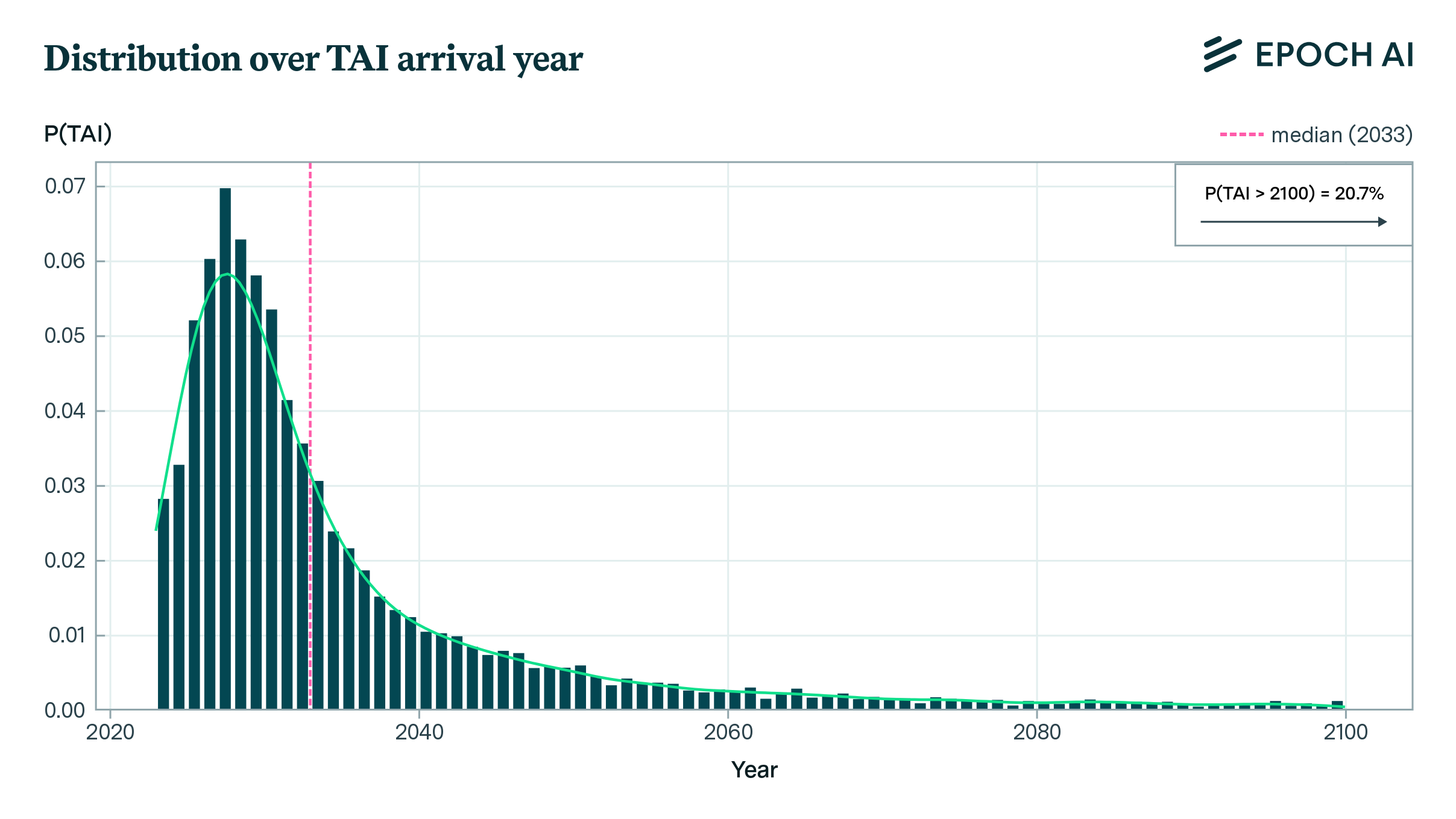
These components are combined to estimate the probability that the compute needs for transformative AI will be met in a given future year. Under default parameter values calibrated on historical estimates, the simple extrapolative model assigns a high chance of the development of transformative AI by 2050.
We take this to mean that current trends of algorithmic progress and compute scaling, if continued, will likely lead to AI systems within several decades that have dramatic effects on scientific progress and economic growth. The outputs of this model should not be construed as the authors’ all-things-considered views on the question of when transformative AI will arrive. Instead, the model is better seen as potentially illustrating the predictions of well-informed extrapolative models.
There have been many attempts to forecast the date at which AI models will achieve human level performance on a transformative task.1 2 We contribute another, making use of our Direct Approach framework (Barnett and Besiroglu, 2023), which uses neural scaling laws to bound the compute needed to train a transformative model. Our work is most similar to Forecasting TAI with biological anchors (Cotra, 2020).
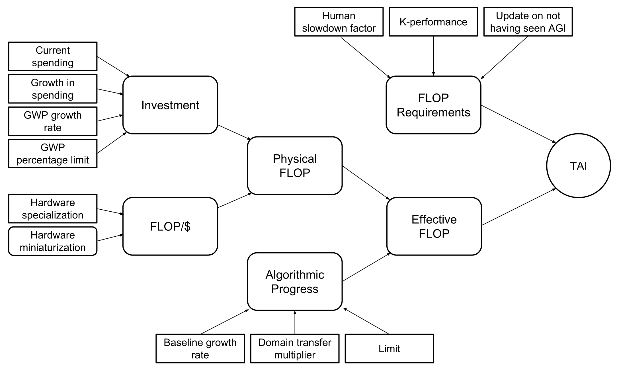
Our forecast model has four user-adjustable components, pictured in the figure below: investment in model training, hardware price performance, algorithmic progress, and the compute requirements produced by the Direct Approach. Together, they produce a probability of TAI being trained during each year. Investment and hardware price performance combine to produce an estimate (which we call “physical FLOP”) of the total FLOP available during a given year. When the amount of physical FLOP is adjusted to account for algorithmic progress, we get an estimate of the amount of “effective FLOP”—the amount of physical FLOP that would be required to reach a given level of performance if algorithms did not improve. Finally, this effective FLOP estimate is compared to the FLOP requirements produced by the Direct Approach. When the number of effective FLOP exceeds those requirements, we consider TAI to have been achieved.
Compute requirements
The compute requirements for human-level AI are generated using our Direct Approach framework, which is an approach based on extrapolating a neural scaling law. This approach requires three parameters, which are explained in more detail in (Barnett and Besiroglu, 2023). Our estimates are intended to provide illustrative and highly speculative guesses for the parameters, taking into account the fact that the Chinchilla scaling law was derived from models trained on internet data, rather than scientific data.
Scaling law. We employ the scaling law estimated by Hoffmann et al., 2022, which takes the form of \(L = E + AN^{-\alpha} + BD^{-\beta}\). The central estimates of the parameters are: A = 306, B = 411, \(\alpha\) = 0.34 and \(\beta\) = 0.28. We model these as the means of normal distributions with standard deviation = 25 for parameters A and B, and standard deviation = 0.05 for \(\alpha\) and \(\beta\).
K-performance. This refers roughly to the average number of tokens generated by a model that a human judge requires in order to reliably distinguish the model’s outputs from a human expert’s outputs, on some task. Our default distribution, generated by an internal poll, is lognormal with an 80% confidence interval of 2,000 to 222,000. This was anchored to the number of tokens in a typical scientific manuscript.3 This reflects our view that producing scientific work indistinguishable from actual scientific work is a strong candidate for a task, which, when mastered by AI, is likely to be transformative.
Slowdown factor. This parameter represents the multiplier for the number of tokens human discriminators will need to see compared to an ideal Bayesian predictor, when distinguishing between human- and computer-generated texts. Informed by an internal poll, we enforce a lognormal distribution with a median of 53.1, a 15th percentile estimate of 9.84, and an 85th percentile of 290. This parameter is perhaps the most subjective of all the parameters considered, as we do not yet have reliable data on how quickly trained human judges can discriminate between real and model-generated texts.
These distributions produce the following distribution over the effective FLOP requirements.4
We apply a further adjustment to the distribution to reflect our observation of having not achieved transformative AI at a level of O(1e25) FLOP, which is commensurate with the compute-intensity of the largest training run to date.5
The Direct Approach framework yields a soft-upper bound, meaning that we can be reasonably confident that the effective compute requirements will not exceed the bound for a given set of parameter values. The reason is that a more efficient means of automating high-quality reasoning may be developed than the method of training large models to emulate human reasoning. However, we think this bound is unlikely to be more than a few orders of magnitude larger than what is required if we assume that deep-learning based autoregressive models remain the dominant approach in AI. To adjust for the fact that this framework produces an upper bound, rather than a central estimate, we have automatically scaled the compute requirements distribution by 5/7 around the point 10^25 to put more probability on lower compute values.6
Algorithmic Progress
Algorithmic progress refers to improvements in the algorithms and architectures of machine learning models that reduce the amount of compute necessary to reach a given level of performance.
We use three parameters to model algorithmic progress:
Baseline rate of efficiency improvements. Erdil and Besiroglu (2022) estimate that the historical rate of algorithmic progress in computer vision models has been 0.4 orders of magnitude per year (80% CI: 0.244 to 0.775).
Domain transfer multiplier. We might well expect the pace of progress towards transformative models to be meaningfully different from that of progress in computer vision algorithms. To account for that, we multiply the baseline growth rate with a parameter—lognormally distributed, with values elicited via an internal poll—representing the extent to which we expect progress in potentially-transformative models to be faster or slower than the rate in computer vision.
Algorithmic progress limit. It’s reasonable to expect that the previously-seen exponential growth in algorithmic efficiency will not continue indefinitely. This parameter addresses this concern by representing the maximum possible performance multiple relative to 2023. The parameter follows a lognormal distribution, with its default interval sourced from an internal poll.
At each timestep, algorithmic efficiency increases at the baseline growth rate times the domain transfer multiplier. As the resulting multiplier reaches the limit, the rate of growth approaches zero.
Investment
Historically, investment in large-scale training runs has grown at between 25.9% and 151.3% per year, over the 2015 to 2022 period (Cottier, 2023a). We model the investment in potentially-transformative training runs by combining estimates of the dollar cost of current training runs, projections of future GWP growth, and estimates for the maximum percentage of GWP that might be spent on such a training run.
Current spending. We estimate that the current largest training run in 2023 will cost $61 million, using our tentative guess at GPT-4’s training cost (Cottier, 2023b), and updating it in line with previous growth rates found in Cottier, 2023a.
Yearly growth in spending. Following Cottier, 2023a, we assume spending will increase between 146% and 246% per year (80% CI).
GWP growth rate. OECD, 2021 projects that world GWP will be $238 trillion in 2060, implying a 1.9% per year growth rate. We use this as the center of 80% CI of 0.400% to 4.75% per year.
Maximum percentage of GWP spent on training. Since spending on training runs is growing faster than GWP, a naive extrapolation suggests that we will eventually see training runs which cost many multiples of GWP. To account for this, we include a parameter that represents the maximum possible share of GWP that can be spent on a training run. We tentatively put this at 0.0137% to 1.46% (80% CI).
As spending approaches the limit defined by the GWP and the GWP percentage limit, growth in spending slows. Eventually, spending growth is entirely limited by the growth of GWP.
Compute
The first aspect of compute we consider is the progress of FLOP/s per dollar. We modify projections of the growth in FLOP/s in top GPUs (Hobbhahn and Besiroglu, 2022) to incorporate an estimate of the benefits from hardware specialization.
The hardware specialization parameter is designed to account for future adjustments for specific workloads, including changes to parallelism, memory optimization, data specialization, quantization, and so on. We assume that gains from such specialization will accrue up until a limit,7 and model the per-year growth of hardware specialization gains with a lognormal distribution, using values elicited from an internal poll.
At each timestep, we use the current rate of FLOP/s growth to estimate the lifetime of a typical GPU. This lifetime, combined with an estimate of the cost of a typical GPU, produces an estimate of the FLOP/$ available at that timestep.8
Using these FLOP/$ figures, along with the projection of spending described above, we can estimate the number of FLOP available each year (“Physical FLOP”).
Conclusion
We combine the estimate of physical FLOP with the previous estimate of the algorithmic progress multiplier to get the number of effective FLOP available by year. This is compared to our estimate of the effective FLOP requirements to compute the probability of TAI per year.
| Probability of TAI by… | ||
|---|---|---|
| 2030 | 2050 | 2100 |
| Quantile | ||
|---|---|---|
| 10% | Median | 90% |
In this model, for each year, we consider Transformative AI (TAI) to have arrived if the number of effective FLOP surpasses the estimate generated by the Direct Approach.
The model implemented here is fundamentally extrapolative, meaning that is based on projections of progress in hardware and software and expansions in investment based on historical data. This is in contrast to more sophisticated models that ‘endogenize’ such processes by having explicit models of the economic processes that drive these trends (such that of Davidson, 2022, implemented by Epoch AI here). While evaluating the differences between these modeling approaches is beyond our scope, it should be noted that extrapolative models could produce wider distributions than endogenous models, and that extrapolative models can tend to overstate the likelihood of especially long timelines.
We thank Daniel Kokotajlo, Carl Shulman and Charlie Giattino for their feedback on a draft of this report. We also thank Ege Erdil, Jaime Sevilla, Pablo Villalobos and the rest of the Epoch AI team for their suggestions and previous research.
Appendix: Simulation specification
To generate our results, we run the model described below many times. Each run, or “rollout,” produces an estimate for the value of each component of the model. The results plotted above report the distribution of the values over the rollouts.
In what follows:
- \(\lambda (D, l, u)\) is a function which renormalizes a probability distribution \(D\) to lie in \((l, u)\)
- The notation \(x \leftarrow D\) is used to indicate that \(x\) is sampled from \(D\).
- The function \(\kappa\), defined as \(\kappa (v, l) = l (1 - \exp(-v/l))\), constrains the value of \(v\) to be no higher than \(l\).
The concrete numbers are chosen to produce distributions which match the default confidence intervals provided by the interactive tool. Lognormal distributions are parameterized with the mean and standard deviation of the underlying normal distribution.
Investment
For each rollout, we start with:
-
\(P_{2023} = 1.17e14\), representing GWP in 2023
-
\(p \leftarrow Lognormal(-1.96, 1.82)\), representing the maximum percentage of GWP that could be spent on a training run
-
\(S_{2022} = 6e7\), representing the maximum dollar amount that could be spent on a training run in 2023
-
\(r_P \leftarrow \lambda(N(2.58 1.70), -1, \infty)\), which operates as the GWP growth rate
-
\(r_S \leftarrow (N(62.7, 22.3), -1, \infty)\), which operates as the growth in spending, before the spending limit is taken into consideration
To update, we use the following equations:
-
\(P_{t+1} = \left( 1 + \frac{r_P}{100} \right) P_t\),
-
\(S_{t+1} = \left( 1 + \frac{r_S}{100} \right) S_t\),
-
\(I_{t+1} = \kappa \left( S_t, \frac{p}{100}P_t \right)\),
where \(l_t\) represents our estimate of investment in year \(t\).
Algorithmic Improvements
For each rollout, we start with:
-
\(a \leftarrow Lognormal(1.65, 0.656)\), representing the largest possible algorithmic improvement, expressed as orders of magnitude
-
\(R_a \sim N(0.550, 0.156)\), representing base projections of algorithmic improvement each year, extrapolating from computer vision and expressed as orders of magnitude
-
\(T_a \sim Lognormal(-0.410, 0.488)\), representing the domain transfer multiplier
-
\(r_a \leftarrow T_a R_a\), representing the growth in algorithmic progress each year
To update, we use the following equation:
- \(A_t = \kappa(10^{(t-2022)r_a}, 10^a)\),
where \(A_t\) represents the estimate of algorithmic progress achieved in year \(t\).
Compute
We use \(E_t\) to represent the baseline projection of FLOP/s for top GPUs found in Hobbhahn and Besiroglu, 2022 at year \(t\). Starting with:
- \(h \leftarrow Lognormal(-2.30, 0.715)\), representing the number of orders of magnitude at which performance grows each year due to hardware specialization
At each timestep, we set
-
\(H_t= E_t \cdot 10^{\max((t-2022)h, \log_{10}(250))}\), representing the baseline FLOP/s projections, updated to account for a capped projection of hardware specialization gains
-
\(D_t = \frac{365 \cdot 24 \cdot 60 \cdot 60 \cdot 1.2}{0.1 + H_t/H_{t-1}}\), representing the number of seconds over which we expect the cost of each GPU to be amortized
-
\(F_t = \frac{H_t D_t}{5000}\), representing the FLOP/$ available at year \(t\), assuming the price for a top GPU to be $5,000
Combined Model
For a given rollout, we say that TAI is achievable in year \(t\) if \(A_t I_t F_t > T\), where \(T\) represents the FLOP requirements for TAI given by the Direct Approach. \(P(\mathrm{TAI\ by\ year}\ t)\) is defined as the percentage of rollouts for which \(A_t I_t F_t > T\).
Notes
-
By a transformative task we imagine tasks like scientific research, which if cheaply automated, we think will likely drastically accelerate economic growth rates. ↩
-
See Wynroe, et al, 2023 for a review. ↩
-
Fire and Guestrin, 2019 analyze 120M scientific papers and find that the average number of pages in 2014 was 8.4. Assuming that there are 500 words per page, and 0.75 tokens/word, this amounts to 5600 tokens/publication. ↩
-
Note that this is effective FLOP instead of physical FLOP, as this is the estimate for the amount of FLOP needed to reach transformative levels of automation with 2023 algorithms. We will address algorithmic progress in a later section of the model. ↩
-
This adjustment was modeled as a Bayesian update for parameter values of a scaling law that defined the arrival rate of transformative AI in a poisson process. The power law has two parameters: a coefficient and an exponent. The exponent is fixed at 0.3, as it merely determines the smoothing of the update. The prior over the coefficient is set such that the prior FLOP requirement distribution defines the scale over which you expect transformative AI to arrive in 1 year. The parameter values were updated on the basis of seeing a series of sequential training runs at various FLOP scales, with the amount of time between training runs. The training run sequences that produced the distribution seen below were: (10^17 FLOP, 8 years), (10^23 FLOP, 2 years), (10^25 FLOP, 1 year). ↩
-
In case the reader does not wish to apply this ad-hoc adjustment, they can disable this scaling by unselecting the “Apply scaling” box in the compute requirements section. ↩
-
The TPU-V1 was on average about 15X-30X faster than its contemporary GPU lacking architectural optimizations for AI workloads (Jouppi et al., 2017), and later versions of the TPU, such as the V3 provide an additional order of magnitude of performance in similar floating point representations per chip. While a large part of the improvements in accelerators is often explained by CMOS scaling (see Fuchs and Wentzlaff, 2018) rather than architectural improvements alone, it is not unlikely that an increase in tensor cores and a reduction in relevant precision could together provide an increase of performance equivalent to increasing FLOP/s by 1 or 2 orders of magnitude in some given floating point precision. In light of this, given that improvements “at the top” are likely to be exhausted in the short-to-medium term, we set a cap of 250x on the additional performance improvements from a continuation of similar architectural improvements. ↩
-
Specifically, at each year, we treat the lifetime of a typical GPU as 1.2/(r+0.1), where r is the value of that year’s growth in FLOP/s. (If hardware is improving quickly at 30% each year, for example, replacement times will be a relatively short three years. In the limit, if hardware improvements stop, replacement times will be longer: 12 years). The GPU lifetime multiplied by the FLOP/s tells us how many FLOP the GPU will make available over its lifetime. Finally, we divide that by the cost of a top GPU to get the FLOP/$, setting the cost of a GPU to $5000 so that it provides 4e17 FLOP/$ in 2023, which is in line with the realized price performance of today’s GPUs used in large-scale training runs. ↩
Updates
Previously, the distribution over TAI arrival year was normalized to 1 in this century, so that the figures showed this distribution conditional on TAI happening within the bounds of the graphs (2023 to 2100). We’re no longer performing this normalization.
We updated our best guesses for the rate of investment growth (previous 80% CI: [34, 91] %/year) and algorithmic progress (previous 80% CI: [0.21, 0.65] OOM/year). The previous guess for investment growth was based on the trend for the very largest training runs, but we now believe anchoring to the trend for all significant training runs in our dataset is a more sound approach.
We fixed a bug that caused the model to produce extremely low TAI requirements in a small percentage of simulations.
Previously, two simulations run consecutively with the same parameters would produce the same result in some cases. We changed the way we seed the simulations to make them independent of each other.
We rewrote a sentence for clarification and fixed a link.
We rewrote some sentences for clarification.
We modified the interactive model to perform an update on the FLOP requirements needed for transformative AI, which more explicitly considers that the framework provides an estimate of the upper bound rather than the actual requirements. See details of this change here.
Previously, our estimate for algorithmic progress was based on an internal poll from Epoch AI researchers (80% CI: [0.35, 0.75] OOM/year). Now, we have grounded it in an estimate for the rate of algorithmic progress in computer vision (Erdil and Besiroglu, 2023).


